Wirujące Szeregi Fouriera
Rozdział 7 Jak obliczać środki ciężkości trajektorii scn?
Rozdział 7.1 Wstęp
W rozdziałach 4,5 i 6 wyłuskaliśmy z wirującej trajektorii F(njω0t) jej “środek ciężkości” sc jako liczbę zespoloną. A to jest już prawie n-ta harmoniczna o pulsacji ω=n*ω0 funkcji f(t), bo scn=2*sc. Wtedy jeszcze nie znaliśmy wzoru na scn i wynik przyjęliśmy bez dowodu. Teraz poznamy go na Rys. 7-2b,c a także związek środka ciężkości scn trajektorii n-tej z n-tą harmoniczną f(t) na Rys. 7-2i,j.
Rozdział 7.2 “Środek ciężkości” trajektorii a harmoniczne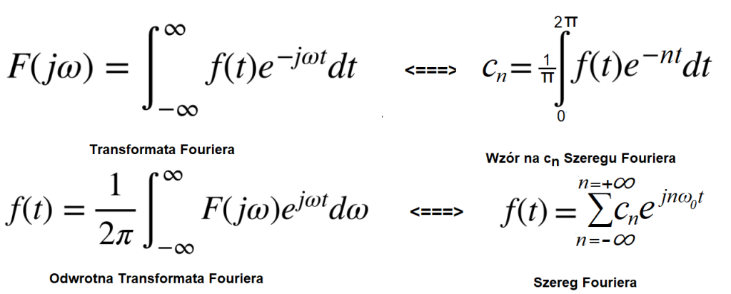
Rys. 7-1
Dziwne wzory
Na razie nie wnikaj w szczegóły. Powiem tylko, że wzory należą do najważniejszych w matematyce, tak jak mckwadrat w fizyce. Nie są intuicyjne, bo czego tu nie ma? Funkcje zespolone, całki, nieskończoności, pulsacje ω. Równania odpowiadają jakimś trajektoriom na płaszczyźnie zespolonej. A tzw. “środek ciężkości” trajektorii bardzo ułatwi zrozumienie tych dziwnych i trudnych wzorów.
Rozdział 7.3 “Środek ciężkości” scn trajektorii F(nj funkcji f(t) obracającej się z prędkością -nω0.
Środkiem ciężkości scn dla n-tej F(njωt) trajektorii jest liczba zespolona, z której łatwo odczytamy harmoniczną funkcji f(t) o pulsacji ω=n*ω0. Tak jakbyśmy do wirówki obracającej się z prędkością ω=n*ω0 wrzucili funkcję okresową f(t). I co z niej wypada? Oczywiście że harmoniczna o pulsacji ω=n*ω0! Do tej pory środek ciężkości scn wyznaczaliśmy intuicyjnie. W prostych przypadkach, gdy scn=(0,0), pokrywało się to z oczekiwaniami. Tak jak np. środek ciężkości okręgu. Teraz przyszedł czas na dokładny wzór na scn. Nie będzie ścisłego dowodu. Natomiast postaram się, żeby było to tak oczywiste, jak jazda na rowerze. Chociaż czy jazda na rowerze jest oczywista? Pierwsi cykliści w XIX wieku byli traktowani jak cyrkowcy. Jak to tak, jedzie i nie przewraca się?
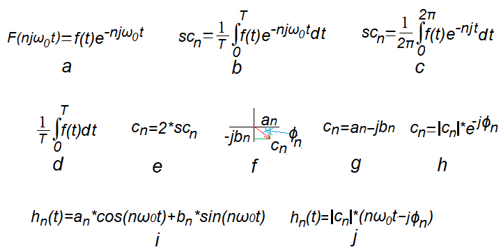
Rys. 7-2
Związek środka ciężkości scn trajektorii F(njω0t) z zespolonymi współczynnikami Fouriera c0, cn=an-jbn* i harmonicznymi hn(t) funkcji f(t) o okresie T.
* Wydaje się, że wzór 7-2g as cn=an+jbn byłby bardziej naturalny. Ale wtedy wzór 7-2i pojawiałby się w Szeregach Fouriera jako hn(t)=an*cos(nω0t)-bn*sin(nω0t).
Rys. 7-2a
Trajektoria F(njω0t)
Punkt porusza się na osi rzeczywistej Re Z zgodnie z funkcją okresową f(t). Gdy wirówka (płaszczyzna Z) z funkcją f(t) obraca się z prędkością -nω0 (znak –, bo “zegarowo”), to rysowana jest trajektoria wg. funkcji zespolonej F(njω0t). Dla n=0 wirówka stoi.
Pojęcie trajektorii jest już dla Ciebie znane po rozdz. 4,5 i 6. Jeżeli coś nie tak, to polecam chociaż p. 4.3 z rozdz. 4.
Rys. 7-2b
Wzór ogólny na środek ciężkości scn trajektorii F(njω0t).
Funkcją podcałkową jest trajektoria F(njω0t). Całkę (podzieloną przez 2T) możemy traktować jako punkt scn średnio odległy trajektorii F(njω0t) od początku współrzędnych (0,0) w okresie T sek*. Wtedy dla n=1 trajektoria F(njω0t) wykona 1 obrót w okresie T=2π/1ω0, dla n=2–> 2 obroty itd… Ale zawsze w tym samym okresie T, tylko z większą prędkością ω!
*Jeżeli taka definicja środka ciężkości trajektorii F(njω0t) nie jest przekonująca, to może pomoże (nawet do rymu) rozdz. 7.7
Rys. 7-2c
Dla funkcji które są “podobne w czasie”, np. fale prostokątne o wypełnieniu 50%, i amplitudach A=1 ale o różnych pulsacjach to środki ciężkości scn nie zależą od pulsacji ω. Są takie same dla ω=1/sek i ω=1000/sek! Dlatego możemy w wzorze Rys. 7-2b założyć ω=1/sek i powstanie wzór uproszczony Rys. 7-2c. Więcej na ten temat w rozdz. 7.6
Rys. 7-2d
Wzór na współczynnik c0 szeregu Fouriera dla n=0.
Jest to składowa stała funkcji f(t) i dlatego jest zawsze liczbą rzeczywistą sc0=c0=a0. Podstaw n=0 do wzoru Rys. 7-2b, to wyjdzie klasyczna średnia funkcji okresowej f(t) w okresie T.
Uwagi dla wzorów 7-2b i 7-2d
Przedziałem całkowania jest 0…T. Ale może też być np. -T/2…+T/2. Ważne żeby przedział miał długość okresu T.
Rys. 7-2e
Wzór na na pozostałe n-te współczynniki szeregu cn Fouriera dla ω=1ω0, ω=2ω0…ω=nω0.
Są to zespolone anplitudy harmonicznych hn(t) jako podwojone środki ciężkości scn. Dlaczego podwojone scn dla n=1,2…,a sc0 jest niepodwojone? Dobre pytanie. Spróbuję odpowiedzieć w rozdz. 12.
Rys. 7-2f
Środek Ciężkości trajektorii jako Liczba zespolona scn, lub wektor o składowych an oraz jbn. Może być przedstawiona w wersji algebraicznej i wykładniczej
Rys. 7-2g
scn w wersji wersji algebraicznej
cn=an-jbn
-cn jest amplitudą zespoloną n-tej harmonicznej nω0
-an amplitudą składowej cosinusoidalnej n-tej harmonicznej o pulsacji nω0
-bn amplitudą składowej sinusoidalnej n-tej harmonicznej o pulsacji nω0
Rys. 7-2h.
cn w wersji wersji wykładniczej
cn=|cn|*exp(+jϕn)
Wyraźnie widać moduł |cn| i fazę ϕn dla pulsacji ω=nω0. Najczęściej sinusoida wyjściowa jest opóźniona względem wejściowej i dlatego ϕn jest ujemne.
Rys. 7-2i
n-ta harmoniczna hn(t) jako suma składowej cosinusoidalnej i sinusoidalnej.
Rys. 7-2j
n-ta harmoniczna hn(t) jako cosinus z przesunięciem fazowym ϕ
Moduł |cn|, inaczej moduł |cn| jest “pitagorasem” z an i bn, zaś tg(ϕ)=bn/an.
A teraz konkret. Jak obliczyć harmoniczne jakiejś funkcji okresowej o znanym wykresie i pulsacji np. ω0=10/sek czyli okresie T=2π/ω0≈0.628 sek?
Po pierwsze. Wiemy już, że jeżeli kształt funkcji w okresie jest znany, to parametry an, bn czyli harmoniczne nie zależą od okresu T funkcji. Niech będzie będzie to np. znormalizowane T=2π sek. Czyli dla ω0=1/sek.
Po drugie. Ze wzoru Rys. 7-2c obliczymy c0=a0 jako wartość średnią funkcji w okresie T=2π sek.
Załóżmy np.
c0=a0=0.5
Po trzecie. Ze wzoru Rys. 7-2c obliczymy środki ciężkości trajektorii scn dla
pulsacji 1ω0, 2ω0,…nω0…
Załóżmy np.
sc1=4-2j dla 1ω0=1/sek
sc3=2-1j dla 3ω0=3/sek
sc5=1+0.5j dla 5ω0=5/sek
Dla pozostałych nω0 środki ciężkości trajektorii scn=0
Uwaga:
Wzór Rys. 7-2c wywołuje zawrót głowy. Całki, liczby zespolone, nieskończoności… Apage Satanas!
Ale od czego mamy Wolfram Alfa. Niech to będzie jego zmartwienie w Rozdz. 11
Po czwarte
Ze wzoru cn=2*scn obliczymy parametry scn dla pulsacji ω=1/sek, ω=2/sek…, ω=n/sek…
w wersji algebraicznej Rys. 7-2f
c1=8-4j
c3=4-2j
c5=2+1j
lub w wersji wykładniczej Rys. 7-2g
c1≈8.94*exp(-j26.6°)
c3≈4.47*exp(-j26.6°)
c5≈2.23*exp(+j26.6°)
Przypominam, że np. 8.94 to to moduł |8-4j| czyli “pitagoras z 8 i 4″ a tg(26.6°)≈4/8.
Po piąte
Teraz możemy przedstawić kolejne harmoniczne h1(t),h2(t),h3(t)…
wg. Rys. 7-2h
h1(t)=8cos(1t)+4sin(1t)
h2(t)=4cos(2t)+2sin(2t)
h3(t)=2cos(3t)-1sin(3t)
lub wg. Rys. 7-2i
h1(t)=≈8.94*cos(1t-26.6°)
h2(t)=≈4.47*cos(2t-26.6°)
h3(t)=≈2.23*exp(3t+26.6°)
No dobrze, ale my chcemy wzory na harmoniczne dla f(t) o pulsacji ω0=10/sek.
Amplitudy zespolone będą takie same czyli:
h1(t)=8cos(10t)+4sin(10t)
h2(t)=4cos(20t)+2sin(20t)
h3(t)=2cos(30t)-1sin(30t)
lub wg. Rys. 7-2i
h1(t)=≈8.94*cos(10t-26.6°)
h2(t)=≈4.47*cos(20t-26.6°)
h3(t)=≈2.23*exp(30t+26.6°)
Rozdział 7.4 “Środki ciężkości” scn trajektorii F(-njω0t) dla różnych funkcji f(t),
Rozdział 7.4.1 Wstęp
Wzór Rys. 7-2a dotyczy trajektorii F(njω0t), gdy płaszczyzna z funkcją f(t) wiruje z różnymi prędkościami ω=n*ω0. Dla n=0 płaszczyzna Z nie wiruje. Trajektoria powinna już być dla Ciebie oczywista, zwłaszcza po animacjach.
Rozpatrzymy wzór Rys. 7-2b na środek ciężkości scn trajektorii F(njω0t) dla różnych funkcji f(t) i różnych prędkości wirowania n*ω0. Następnie zbadamy związek środków ciężkości scn z kolejnymi harmonicznymi hn(t) funkcji f(t).
Zbadamy kolejne funkcje zaczynając od najprostszej.
1. f(t)=1–> Rozdział 7.4.2
2. f(t)=0.5cos(4t) Rozdział 7.4.3
3. f(t)=1.3+0.7*cos(2t)+0.5*cos(4t) Rozdział 7.4.4
4. f(t)=0.5+1.08*cos(1t-33.7°)+0.72*cos(3t+33.7°)+0.45*cos(5t-26.6°) Rozdział 7.4.5
Główne wnioski:
1. Wzór Rys.7-2b wskazuje punkt scn na płaszczyźnie Z, który jest średnioodległy między z=(0,0) a trajektorią F(njω0t), gdy płaszczyzna Z wykona n obrotów 0…2π. Innymi słowy, punkt scn jest jakby “środkiem ciężkości” trajektorii F(njω0t).
“Jakby”? Bo prawdziwy środek ciężkości jest obliczany wg. innych wzorów niż na scn, chociaż czasem się pokrywają.
2. Ze środka ciężkości scn trajektorii łatwo obliczymy n-tą harmoniczną funkcji f(t) dla n*ω0. W naszych przykładach ω0=1/sek.
W rozdziale 11 sprawdzimy programem WolframAlfa wzory z Rys.7-2. Wtedy jeszcze bardziej przekonasz się, że wzory Rys. 7-2 są oczywiste jak jazda na rowerze.
Rozdział 7.4.2 Środki ciężkości scn trajektorii F(-njω0t)
dla funkcji f(t)=1
gdy n=1 i ω0=1/sek
Zaczniemy od najprostszego przypadku tj. funkcji stałej f(t)=1.
Odpowiedź jest oczywista bez wzorów.
1. Funkcja nie ma żadnych harmonicznych. Czyli środki ciężkości scn trajektorii dla każdej pulsacji n*ω0 powinny być zerowe tj. scn=(0,0).
2. Składowa stała c0=a0=1.
Sprawdzimy czy wzory Rys. 7-2c i 7-2d to potwierdzą.
Zbadamy trajektorię F(njω0t) dla f(t)=1, n=1 i ω0=1/sek wg. wzoru Rys. 7-2a.
Niektórzy mogą kręcić nosem czy f(t)=1 jest funkcją okresową? Jest, bo co okres T (nawet dowolne T!) funkcja się powtarza
Rys. 7-3
Funkcja zespolona 1exp(-1j1t) jako trajektoria i jej “środek ciężkości” sc1.
Rys. 7-3a
Funkcja zespolona 1exp(-1j1t) jako wirujący wektor.
Kliknij. W ciągu okresu T=2π/ω≈6.28sek wektor wykona jeden obrót. A gdybyśmy w czasie obrotu sumowali kolejne wektory?
Rys. 7-3b
Okrąg jako ślad po wirującym wektorze czyli trajektoria 1exp(-1j1t).
Już bez obliczeń wiemy, że środkiem ciężkości jest scn=(0,0). Czy wzór Rys.7-3c to potwierdzi?
Widzisz kolejne położenia wektorów od z0, z1… z11 przy przyroście kąta -Δωt=-30º. Ich sumą jest wektor zerowy z=(0,0). Dlaczego zerowy? Bo każdemu wirującemu wektorowi odpowiada wektor kompensujący (np. z4 i z10) i ich suma jest zerowa. Czyli suma wszystkich wektorów z=(0,0) jest jakby “środkiem ciężkości” trajektorii funkcji zespolonej 1exp(jωt). Ściślej, aby otrzymać średnią odległość, to należy jeszcze podzielić sumę wektorów, czyli z=(0,0) przez 12*30º=360º, inaczej przez 2π.
Rys. 7-3c
Dokładniejszy wzór na środek ciężkości scn trajektorii funkcji zespolonej 1exp(-1jω0t) dla ω0=-1/sek
Wyrażenie α=-ω0*t jest wirującym z prędkością ω0=1/sek kątem α.
Definicja środka ciężkości z Rys. 7-3b jako sumy 12 wektorów nie była zbyt precyzyjna. Przyrostem kąta jest Δα=30º . A przecież jest nieskończenie wiele, nieskończenie małych przyrostów Δα=d(ωt) od α=0 do α=2π. Sumowanie zmieni się w całkowanie od 0 do 2π.
A skąd dzielenie przez 2π? Jest konieczne do obliczenia średniej odległość trajektorii przy obrocie 0…2π od początku współrzędnych (0,0). Tu akurat średnia i suma wektorów są równe z=(0,0).
Jeszcze jedno. Wektory na Rys. 7-2b odpowiadają siłom odśrodkowym. Inaczej “rozrywającym” okrąg. Tak czy owak to punkt przyłożenia wypadkowej tych sił F, tu akurat z=(0,0) leży dokładnie w punkcie scn=(0,0) płaszczyzny zespolonej.
Wnioski
Z trajektorii 1exp(-1j1t) wynika jej sc1=(0,0) dla ω=-1/sek. Czyli harmoniczna o pulsacji ω=1/sek na podstawie wzoru Rys. 7-2c też jest zerowa! A gdyby wirówka pracowała z innymi prędkościami ω? Wtedy też scn=(0,0). Czyli funkcja stała f(t)=1 nie ma żadnej harmonicznej, a tylko składową stałą c0=a0=1. Niezbyt to odkrywcze, ale dzięki temu dla prostej funkcji f(t)=1 wzory z Rys. 7-2 są oczywiste. I o to chodzi!
Rozdział 7.4.3 Środki ciężkości scn trajektorii F(-njω0t) dla funkcji
f(t)=0.5cos(4t)
gdy n=0,1,2,…8 i ω0=1/sek
Zbadamy trajektorie F(njω0t)=f(t)*exp(-njω0t) dla:
f(t)=0.5cos(4t)
n=0,1,2 …8
ω0=1/sek
Rys. 7-4
Funkcje zespolone F(n1t)=0.5cos(4t)*exp(-n1t) jako trajektorie i jej “środki ciężkości” scn.
ω=0 (n=0)
Nieruchoma płaszczyzna zespolona Z, na której funkcja f(t)=0.5cos(4t) wykonuje ruchy harmoniczne “wte i we wte”.
ω=4/sek (n=4)
Tylko przy tej prędkości ω powstanie trajektoria z niezerowym środkiem ciężkości sc4=(0.25,0). Intuicja podpowiada, że jest on średnioodległy od z=(0,0) i taki wynik obliczymy wzorem Rys. 7-2c. Zauważ, że ruch trajektorii widzisz tylko na początku. Potem odbywa się po tym samym torze i dlatego trajektoria jest pozornie nieruchoma.
Pozostałe ω (n=1,2, 3, 5, 7, 8)
Środki ciężkości scn=(0,0), które też podpadają pod wzór Rys. 7-2b.
Składowa stała c0.
Ewidentnie potwierdza wzór Rys.7-2d–> sc0=(0,0)=a0==0.
Czwarta harmoniczna h4(t) czyli dla ω=4/sek
wg. Rys. 7-2e–>c4=2*sc4=2*(0.25,0)=(0.5,0)=0.5+j0–>a4=0.5 i b4=0
wg. Rys. 7-2i–>h4(t)=0.5*cos(4t)
Harmoniczne dla pozostałych pulsacji n*ω0 nie istnieją, bo środki ciężkości scn ich trajektorii są zerowe.
Wniosek
Funkcja f(t)=0.5*cos(4t) składa się tylko z jednej harmonicznej h4(t)=0.5*cos(4t). Nie jest to odkrycie Ameryki, ale nam chodzi głównie o potwierdzenie wzorów Rys.7-2.
Uwaga:
Tu założyłem, że funkcja f(t)=0.5cos(4t) składa się tylko z jednej tj. czwartej harmonicznej h4(t)=0.5cos(4t) gdzie pierwsza harmoniczna dla 1ω0=1/sek i pozostałe dla 2ω0=2/sek, 3ω0=3/sek, 5ω0=5/sek, 6ω0=6/sek, czyli h1(t)=h2(t)=h3(t)=h5(t)=h6(t)=…=0 są zerowe.
Równie dobrze, i może bardziej naturalne jest, że funkcja f(t)=0.5cos(4t) składa się tylko z jednej pierwszej harmonicznej h1(t)=0.5cos(4t), pozostałe dla 2ω0=8/sek, 3ω0=12/sek, 4ω0=16/sek, 5ω0=20/sek,… są zerowe.
Rozdział 7.4.4 Środki ciężkości scn trajektorii F(-njω0t)
dla funkcji f(t)=1.3+0.7*cos(2t)+0.5*cos(4t)
gdy n=0,1,2,4 i ω0=1/sek
Funkcja f(t) ma 2 harmoniczne tj. 0.7*cos(2t) oraz 0.5*cos(4t) i składową stałą c0=1.3. Ciekawe jak zostaną one “odwirowane”?
Zbadamy trajektorie F(njω0t)=f(t)*exp(-njω0t) dla:
f(t)=1.3+0.7*cos(2t)+0.5*cos(4t)
n=0,1,2 i 4
ω0=1/sek
Będą to więc trajektorie dla ω=0, ω=1/sek, ω=2/sek i ω=4/sek.
Pozostałe trajektorie tj. dla n=3,5,6,7 i 8 wirują, podobnie jak dla n=1 wokół
środka ciężkości scn=(0,0) i ich nie badamy. Możesz je zresztą zobaczyć w rozdziale 5.
Rys. 7-5
Funkcje zespolone F(nj1t)=[1.3+0.7*cos(2t)+0.5*cos(4t)]*exp(-nj1t) jako trajektorie i jej środki ciężkości scn.
ω=0
Nieruchoma zespolona płaszczyzna Z na której funkcja f(t)=1.3+0.7*cos(2t)+0.5*cos(4t) wykonuje ruchy “wte i we wte” wokół sc0=(1.3,0) i który jest składową stałą c0=a0=1.3 funkcji f(t).
ω=2/sek, ω=4/sek,
Przy tych prędkości ω powstaną trajektorie z niezerowymi środkami ciężkości sc2=(0.35,0) i sc4=(0.25,0). Są one średnio odległymi między punktami trajektorii F(2j1t) i F(4j1t) a z=(0,0). Innymi słowy są to “jakby” (bo nie do końca pod względem mechaniki) środki ciężkości tych trajektorii, które obliczymy wzorem Rys. 7-2c.
ω=1/sek i pozostałe ω
Środek ciężkości sc1=(0,0) i pozostałe też podpadają pod wzór Rys. 7-2c
Składowa stała c0.
wg. wzoru Rys.7-2d–> c0=a0=1.3
Jest to także środek ciężkości sc0=(1.3,0) dla ω=0
Druga harmoniczne h2(t) czyli dla ω=2/sek
wg. Rys. 7-2e–>c2=2*sc2=2*(0.35,0)=(0.7,0)=0.7+j0–>a2=0.7 i b2=0
wg. Rys. 7-2i–>h2(t)=–>0.7*cos(4t)
Czwarta harmoniczne h4(t) czyli dla ω=4/sek
wg. Rys. 7-2e–>c4=2*sc4=2*(0.25,0)=(0.5,0)=0.5+j0–>a4=0.5 i b4=0
wg. Rys. 7-2i–>h4(t)=–>0.5*cos(4t)
Pozostałe harmoniczne nie istnieją, bo środki ciężkości ich trajektorii są zerowe.
Rozdział 7.4.5 Środki ciężkości sc trajektorii F(-njω0t)
dla funkcji f(t)=0.5+1.08*cos(1t-33.7°)+0.72*cos(3t+33.7°)+0.45*cos(5t-26.6°)
gdy n=0,1,2,3,5 i ω0=1/sek
Funkcja f(t) o okresie T=2πsek składa się z trzech cosinusoid z różnymi amplitudami A i fazami ϕ oraz ze składowej stałej c0.
Rys. 7-6
f(t)=0.5+1.08*cos(1t-33.7°)+0.72*cos(3t+33.7°)+0.45*cos(5t-26.6°)
W Rozdziale 6 badaliśmy 9 trajektorii F(-njω0t) funkcji f(t) dla n=0,1,2,…8 i ω0=1/sek.
Jest ona o tyle ciekawa, że ze względu na przesunięcia fazowe ϕ, środki ciężkości scn są liczbami całkowicie zespolonymi.
Każdą harmoniczną można rozłożyć na na składową cosinusoidalną i sinusoidalną i wtedy:
f(t)=0.5+0.9*cos(1t)+0.6*sin(1t)+0.6*cos(3t)-0.4*sin(3t)+0.4*cos(5t)+0.2*sin(5t).
Jest to ta sama funkcja, ale tu łatwo wyznacza się zespolone współczynniki Fouriera, inaczej zespolone amplitudy Fouriera.
Z nich odczytuje się harmoniczne jako przebiegi czasowe h1(t),h3(t) i h5(t) o składowych sinus/cosinus.
c1=0.9-j0.6—>h1(t)=0.9*cos(1t)+0.6*sin(1t)≈1.08*cos(1t-33.7°)
c3=0.6+j0.4–>h3(t)=0.6*cos(3t)-0.4*sin(3t)≈0.72*cos(3t+33.7°)
c5=0.4-j0.2—>h5(t)=0.4*cos(5t)+0.2*sin(5t)≈0.45*cos(5t-26.6°)
Funkcję f(t) włożymy do wirówki z różnymi prędkościami nω0=n*1/sek.
Włączmy obroty na n=0, 1,2,3 i 5, czyli na prędkości ω=0 (wirówka stoi!), ω=-1/sek ,ω=-2/sek, ω=-3/sek i ω=-5/sek. Powstaną trajektorie F(nj1t) tych n którym odpowiadają środki ciężkości scn.
Rys. 7-7
Trajektorie F(nj1t)=[0.5+1.08*cos(1t-33.7°)+0.72*cos(3t+33.7°)+0.45*cos(5t-26.6°)]*exp(-nj1t) dla n=0,1,2,3,5
n=0—>ω=0–>F(0j1t)
Funkcja f(t)=0.5+1.08*cos(1t-33.7°)+0.72*cos(3t+33.7°)+0.45*cos(5t-26.6°) wykonuje ruchy “wte i we wte” wokół sc=(0.5,0) na nieruchomej płaszczyźnie Z. Punkt sc0 jest składową stałą c0=0.5 funkcji f(t).
dla n=1,3,5 czyli dla ω=1/sek, ω=3/sek i ω=5/sek–>F(1jt),F(3jt),F(5jt)
Trajektorie z niezerowymi środkami ciężkości sc1=(0.45,-0.3), sc3=(0.3,+0.2) i sc5=(0.2,-0.1). Punkty te scn są średnio odległymi między punktami trajektorii F(nj1t) a z=(0,0). Innymi słowy są to środki ciężkości scn tych trajektorii, które obliczymy wzorem Rys. 7-2c.
dla n=2 czyli dla ω=2/sek–>F(2jt)
Środek ciężkości sc2=(0,0) też podpada pod wzór Rys. 7-2c. Trajektorii F(4jt), F(5jt), F(6jt), F(7jt), F(8jt) z też zerowymi środkami ciężkości scn nie pokazano.
Składowa stała c0.
wg. wzoru Rys.7-2c–> c0=0.5
Pierwsza harmoniczne h1(t) czyli dla ω=1/sek
wg. Rys. 7-2e–>c1=2*sc1=2*(0.45,-0.3)=0.9+j0.6–>a1=0.9 i b1=0.6
wg. Rys. 7-2i–>h1(t)=–>0.9*cos(1t)+0.6*sin(1t)
wg. Rys. 7-2j–>h1(t)≈–>1.08*cos(1t-33.7°)
Trzecia harmoniczne h3(t) czyli dla ω=3/sek
wg. Rys. 7-2e–>c3=2*sc3=2*(0.3,+0.2)=0.6-j0.4–>a3=0.6 i b3=-0.4
wg. Rys. 7-2i–>h3(t)=–>0.6*cos(3t)-0.4*sin(3t)
wg. Rys. 7-2j–>h3(t)≈–>0.72*cos(3t+33.7°)
Piąta harmoniczne h5(t) czyli dla ω=5/sek
wg. Rys. 7-2e–>c5=2*sc5=2*(0.2,-0.1)=0.4+j0.2–>a5=0.4 i b4=0.2
wg. Rys. 7-2i–>h5(t)=–>0.4*cos(5t)+0.4*sin(5t)
wg. Rys. 7-2j–>h5(t)≈–>0.45*cos(5t-26.6°)
Pozostałe harmoniczne czyli dla np. ω=2/sek, ω=4/sek, ω=6/sek, ω=8/sek, ω=8/sek…
Nie istnieją, bo środki ciężkości scn tych trajektorii są zerowe.
Rozdział 7.5 Detektor harmonicznych
Rozdział 7.5.1 Wstęp
Wiemy już, że n-tej trajektorii F(njω0t) funkcji okresowej f(t) o pulsacji podstawowej ω0 odpowiada środek ciężkości scn, który już jest prawie n-tą harmoniczną f(t).
Dlaczego prawie?
Bo scn nie jest jeszcze n-tą harmoniczną funkcji f(t), ale tylko zespolonym współczynnikiem, z którego łatwo obliczymy n-tą harmoniczną w postaci zespolonej i rzeczywistej.
1. cn=2*scn=an-jbn
2. An=cn=an-jbn jest zespoloną amplitudą n-tej harmonicznej hn(nω0t)
3.a
n-ta harmoniczna w wersji zespolonej
Czyli obracający się z prędkością n*ω0 wektor hn(jn*ω0t)=(an-jbn)*exp(n*jω0t)
3.b
n-ta harmoniczna w wersji rzeczywistej
hn(t)=an*cos(nω0t)+bn*sin(nω0t)–>Rys.7.2i
lub
hn(t)=|cn|*cos(nω0t+ϕ)–>Rys.7.2j
Środki ciężkości scn różnych trajektorii Fn(jnω0t) dla różnych funkcji f(t) znaleźliśmy na Rys. 7-4, Rys. 7-5 i Rys. 7-7. To są “już prawie” n-te harmoniczne f(t).
Przedstawimy teraz te animacje w wersji uproszczonej, tzn.
– będą tylko podwojone środki ciężkości scn dla n-tych trajektorii jako współczynniki cn
– Animacje będą przedstawiane kolejno co 1 sekundę, gdy ω zmienia się od ω=0 do ω=8/sek
W ten sposób powstaną detektory harmonicznych funkcji okresowych f(t) a mianowicie:
Detektor harmonicznych dla:
– f(t)=0.5cos(4t)
– f(t)=1.3+0.7cos(2t)+0.5cos(4t)
– f(t)=0.5+1.08*cos(1t-33.7°)+0.72*cos(3t+33.7°)+0.45*cos(5t-26.6°)
Uwaga:
W poniższych animacjach Detektor=Szukacz
Rozdział 7.5.2 Detektor harmonicznych dla f(t)=0.5cos(4t)
Rys.7-8
Detektor harmonicznych dla f(t)=0.5cos(4t)
Wkładasz do wirówki funkcję okresową f(t)=0.5cos(4t), która wiruje z kolejno zwiększającą się prędkością od ω=0 do ω=8/sek. W ten sposób dla każdej pulsacji ω obliczona jest wg, wzorów z Rys.7-2 kolejna harmoniczna hn(t) której odpowiada liczba zespolona cn. Tu jest tylko jedna harmoniczna niezerowa
dla h4(t)=0.5cos(4t) jako wektor c4=(0.5,0)=0.5. Pozostałe cn=0, czyli odpowiednie harmoniczne nie występują!
Rozdział 7.5.3 Detektor harmonicznych dla f(t)=1.3+0.7cos(2t)+0.5cos(4t)
Rys.7-9
Detektor harmonicznych dla f(t)=1.3+0.7cos(2t)+0.5cos(4t)
Dla ω=0 składowa stała c0=1.3
Dla ω=2/sek c2=0.7 odpowiadająca harmonicznej h2(t)=0.7cos(2t)
Dla ω=4/sek c4=0.5 odpowiadająca harmonicznej h4(t)=0.5cos(4t)
Pozostałe harmoniczne nie występują.
Rozdział 7.5.4 Detektor harmonicznych dla f(t)=0.5+1.08*cos(1t-33.7°)+0.72*cos(3t+33.7°)+0.45*cos(5t-26.6°)
Rys.7-10
Detektor harmonicznych dla f(t)=0.5+1.08*cos(1t-33.7°)+0.72*cos(3t+33.7°)+0.45*cos(5t-26.6°)
Dla ω=0 składowa stała c0=0.5
Dla ω=1/sek c1=1.08*exp(-j33.7°) odpowiadająca harmonicznej h1(t)=1.08*cos(1t-33.7°)
Dla ω=3/sek c3=0.72*exp(+j33.7°) odpowiadająca harmonicznej h3(t)=0.5cos(4t)0.72*cos(3t+33.7°)
Dla ω=5/sek c5=0.45*exp(-j33.7°) odpowiadająca harmonicznej h5(t)=0.45*cos(5t-26.6°)
Pozostałe harmoniczne nie występują.
Uwaga:
Detektory harmonicznych w rozdz. 7.5 badają harmoniczne w zakresie ω=0…+∞. W Szeregach i w Transformacie Fouriera częściej jednak zakłada się, że ω=-∞…0…+∞. Czyli dla pulsacji ω ujemnych i dodatnich. Detektor dla nich został ujęty w artykule “Transformata Fouriera” rys. 5-5.
Rozdział 7.6 Dlaczego “rozciąganie i ściskanie” funkcji okresowej f(t) nie wpływa na parametry an i bn Szeregu Fouriera?
Spójrz na wzory Rys. 7-2b i Rys. 7-2c. Okazuje się, że jeżeli f(t) jest tylko “rozciągnięte/ściśnięte” w czasie (ale nie w pionie!), to wzory nie zależą od okresu T.
Niech naszą funkcją okresową będzie np. f(t)=0.5+1.08*cos(1*1.75t-33.7°)+0.72*cos(3*1.75t+33.7°)+0.45*cos(5*1.75t-26.6°).
Czyli jest to f(t) z Rys.7-6 “ściśnięta” w czasie przez 1.75.
Rys. 7-11
Funkcja okresowa z Rys.7-6, tylko “ściśnięta” w czasie, oraz jej 2 trajektorie.
Rys. 7-11a
Funkcja f(t) na Rys.7-6 miała pulsację ω0=1/sek (T=2π sek), teraz ω0=1.3/sek (T≈3.59sek). Jest “ściśnięta” w czasie przez 1.75.
Rys. 7-11b
Trajektoria F(1jω0t), czyli dla obrotów 1*ω0=1*1.3/sek.
Jest dokładnie taka sama jak na Rys. 7-7 ω=1/sek. Tylko prędkość trajektorii jest 1.3 razy większa.
Wniosek:
Środek ciężkości sc1 trajektorii F(1jω0t) i c1=0.9-j0.6 też będą takie same.
Rys. 7-11c
Trajektoria F(2jω0t), czyli dla obrotów 2*ω0=2*1.3sek.
Jest dokładnie taka sama jak na Rys. 7-7 ω=2/sek.. 6. Tylko prędkość trajektorii jest 1.3 razy większa.
Wniosek:
Środek ciężkości sc2=0 trajektorii F(1jω0t) i c2=(0,0) też będą taka same. Funkcja okresowa f(t) nie ma harmonicznej o pulsacji ω=2*1.3/sek.
W ten sposób moglibyśmy sprawdzić wszystkie pozostałe trajektorie dla ω=3*1.3/sek, ω=4*1.3/sek…ω=8*1.3/sek.
Kształty i środki ciężkości scn będą oczywiście takie same jak w rozdz. 6.
Czyli do obliczania środków ciężkości scn trajektorii, wystarczy “ograniczony” wzór Rys. 7-2c gdy T=2π.
Czyli współczynniki co, c1, c2…cn Szeregu Fouriera nie zależą od okresu T funkcji f(t).
Rozdział 7.7 Dlaczego środek ciężkości scn trajektorii F(njω0t) jest albo:
1-scn=(0,0)-zerowy?
2-scn=(an,bn)-połową amplitudy dla n-tej harmonicznej czyli cn/2?
Każda funkcja f(t) o okresie T czyli pulsacji ω0 składa się ze składowej stałej c0=a0 i harmonicznych o pulsacjach nω0 dla n=1,2,…∞.
-Gdy trajektorie F(n*jω0t)=f(t)*exp(-n*jω0t) wirują z prędkością ω≠nω0, czyli różną od ω każdej harmonicznej, to powstaje sytuacja podobna do animacji Rys. 7-4 ω≠-4. Wtedy trajektorie wszystkich harmonicznych wirują każde z osobna wokół sc=(0,0). Czyli F(n*jω0t) jako ich suma też będzie wirowała wokół sc=(0,0). Czyli przypadek 1-scn=(0,0)-zerowy
-Gdy trajektorie F(n*jω0t)=f(t)*exp(-j*jω0t) wirują z prędkością ω=nω0, czyli równą n-tej harmonicznej, to powstaje sytuacja podobna do animacji Rys. 7-4 ω=-4. Wtedy trajektorie ω≠nω0 pozostałych harmonicznych wirują każde wokół swojego sc=(0,0). A tylko jedna harmoniczna ω=nω0 wiruje wokół scn. Spowoduje to przesunięcie środka ciężkości wszystkich harmonicznych właśnie do tego scn. Czyli przypadek 2-scn=(an,bn)-połową amplitudy dla n-tej harmonicznej czyli cn/2.
Jeszcze jedno. Na animacji Rys.7-4 trajektorie obracały się z prędkościami ω=nω0. Czyli z nie dowolnymi! Natomiast w rozważaniach zakładaliśmy, że są dowolne tylko ω≠nω0. czyli np. ω=-0.384*1/sek. Ale chyba jest oczywiste, że gdy f(t) nie ma harmonicznej dla ω=-0.384*1/sek, to trajektorie F(n*jω0t)=f(t)*exp(-n*j0.384t) też będą wirować wokół scn=(0,0).