Podstawy automatyki
Rozdz. 2 Człon proporcjonalny
Rozdz. 2.1 Wstęp
Zbadamy najprostszy człon dynamiczny- człon proporcjonalny. Wyjście związane jest z wejściem zależnością y(t)=k*x(t). Dlatego rozdział jest raczej pretekstem do zapoznania z animacjami, które najbardziej intuicyjnie przedstawiają człony dynamiczne. Potem łatwiej zrozumiesz aparat matematyczny opisujący człony dynamiczne, czyli równania różniczkowe i transmitancje G(s).
W kolejnych lekcjach mogą pojawić się animacje z którymi postępujemy podobnie:
1. Włączamy video związane z danym członem dynamicznym lub układem regulacji automatycznej.
2. Sygnał wejściowy x(t) może pochodzić z:
– generatora sygnału skokowego (najczęściej)
– wirtualnego suwaka-inaczej sygnał ręczny.
– generatora sygnału liniowego – inaczej “piła”,
– generatora impulsu Diraca – inaczej “krótkie uderzenie młotka”,
3. Obserwujemy sygnał wyjściowy y(t) przy pomocy:
– oscyloskopu (najczęściej)
– bargrafu czyli miernika analogowego,
– miernika cyfrowego,
Obserwowane będą także inne sygnały, np. uchyb regulacji e(t).
Doświadczenia powtarzamy przy różnych parametrach obiektu i różnych sygnałach wejściowych. W efekcie będziesz kojarzył transmitancję G(s) z ich odpowiedziami y(t) na sygnał wejściowy x(t) – najczęściej skok jednostkowy. A bardziej ogólnie – z ich własnościami dynamicznymi.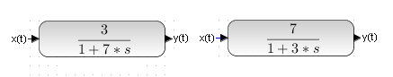
Rys.2-1
Rzucisz tylko okiem na dwie podobne transmitancje G1(s) i G2(s) i od razu będziesz wiedział w czym rzecz.
I to bez znajomości rachunku różniczkowego i operatorowego! Inna rzecz, że wiedza ta nie zaszkodzi.
Rozdział 2.2 Obsługa video
Główną zaletą tego kursu jest animacja obsługiwana przez video. O wiele bardziej działa na wyobraźnię niż zwykły wykres.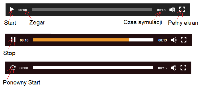
Rys. 2-2
Opis przyciski i wskaźników video
-Start kliknięcie uruchamia animację i zmienia się w przycisk Stop
-Zegar aktualny czas eksperymentu, także jako żółty pasek
-Czas symulacji inaczej-czas trwania eksperymentu.
-Pełny ekran kliknięcie powiększa ekran, ponowne kliknięcie zmniejsza itd…
-Stop Kliknięcie zatrzymuje symulację i zmienia się w przycisk Ponowny Start
-Ponowny Start jak sama nazwa wskazuje.
Rozdział 2.3 Animacja członu proporcjonalnego G(s)=1
Rys.2-3
Animacja członu proporcjonalnego G(s)=1
Kliknij przycisk “Start”.
x(t)-sygnał wejściowy widoczny na suwaku i na mierniku cyfrowym
y(t)-sygnał wyjściowy widoczny na bargrafie i mierniku cyfrowym
Rysunek przedstawia stan początkowy w którym x(t)=0 i y(t)=0 i dlatego bargraf jest niewidoczny. Bargraf jest miernikiem analogowym w postaci pionowego paska o wysokości proporcjonalnej do wielkości mierzonego sygnału y(t).
Nie próbuj poruszać suwakiem! Zrobił to za Ciebie autor i nagrał na video.
Transmitancją G(s) to po prostu wzmocnienie k=1. Zauważ, że reakcja członu proporcjonalnego jest natychmiastowa.
A jaka będzie animacja członu G(s)=2? Wskazania bargrafu i miernika cyfrowego y(t) będą po prostu 2 razy większe.
Rozdz. 2.4 Człon proporcjonalny transmitancji k=1 z suwakiem i oscyloskopem
Na oscyloskopie dwukanałowym będziesz obserwował wejście x(t) i wyjście y(t). Sygnał wejściowy x(t) jest też “machaniem suwaka”.
Rys. 2-4
Przebiegi x(t) i y(t) członu proporcjonalnego G(s) na oscyloskopie dwukanałowym. Z oscyloskopu wynika, że do ok. 17sekundy x(t)=0. Dopiero potem zaczęło się machanie suwaka. Dla członu proporcjonalnego reakcja na wejście jest natychmiastowa, a gdy k=1 to wyjście y(t) jest kopią wejścia x(t).
Rozdz. 2.5 Podsumowanie
Reakcja członu proporcjonalnego jest natychmiastowa. Przy pierwszym podejściu prawie każdy człon dynamiczny jest dla nas członem proporcjonalnym! Nawet omówiony później człon oscylacyjny*. Jak ustawisz temperaturę pieca na +120°C, to po np. 10 min termometr też pokaże +120°C. Czyli transmitancja tego członu G(s)=1. Wejście równa się wyjściu. Tyle tylko, że pomijamy wtedy stan przejściowy! Gdybyś obserwował przebieg czasowy tego pieca na wykresie który obejmuje 24 godziny (a nie 10 min) i oś czasu była tej samej długości jak dla 10 min, to nie widziałbyś stanu przejściowego! Dla Ciebie odpowiedź na skok też byłaby skokiem!
*Uwaga: Nie dotyczy tzw. członów astatycznych np. całkującego. Wrócę jeszcze do tematu