Wirujące Szeregi Fouriera
Rozdział 3 Sumowanie wirujących wektorów exp(jωt)
Rozdział 3.1 A po co to?
Żeby ułatwić zrozumienie sumowanie funkcji cos(ωt), szerzej-funkcji sinusoidalnych.
A to jak znalazł pasuje do Szeregów Fouriera, które są sumą sinusów i cosinusów.
Rozdział 3.2 Ogólnie o sumowaniu wirujących wektorów exp(jωt)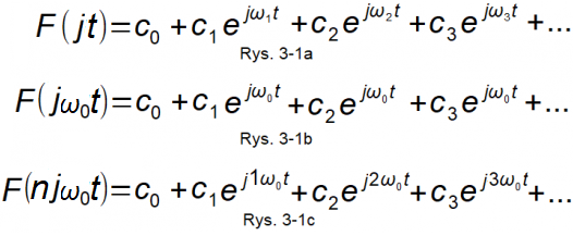
Rys.3-1
Rys.3-1a
Suma wirujących wektorów F(jt) gdzie :
c0 jest składową stałą albo inaczej wirującym wektorem z prędkością ω=0
c1, c2, c3… jest liczbą zespoloną będącą stanem początkowym każdego wektora wirującego c1*exp(jω1t), c2exp(jω2t),ec3xp(jω3t)…
ω1, ω2, ω3… Pulsacje ω1, ω2, ω3… są dowolne! Tzn. mogą ale nie muszą być wielokrotnościami pierwszej harmonicznej ω1. Jest to najbardziej ogólny wzór na sumę i nie będziemy analizować tego przypadku.
Rys.3-1b
Suma wirujących F(jω0t) wektorów z taką samą pulsacją ω0.
Jest nią wektor-liczba zespolona c=c1+c2+c3+…wirujący z prędkością ω0.
Liczba rzeczywista c0 jest składową stałą.
Suma sinusoid i cosinusoid też jest sinusoidą o takiej samej pulsacji ω0 i odpowiednim przesunięciu fazowym φ.
Ma zastosowanie w klasycznej elektrotechnice, gdzie elektrownie wytwarzają prąd o stałej częstotliwości f=50Hz czyli ω0=314*1/sek.
Temat został już dokładnie rozpracowany, chyba jeszcze w XIX wieku.
Przykład z animacją w rozdziale 3.3
Rys.3-1c
Tym głównie będziemy się zajmować.
Tzn. sumą wirujących wektorów F(njω0t) ze zwiększającymi się pulsacjami 1ω0,2ω0, 3ω0…
Podkreślam, że każda pulsacja jest wielokrotnością pulsacji podstawowej nω0, a nie dowolną ω1, ω2, ω3… jak na Rys. 3-1a
Przykłady z animacją w rozdziałach 3.4…7
Rozdział 3.3 Suma 2 wirujących wektorów exp(jωt) o tej samej pulsacji ω0=1/sek
Rozdział 3.3.1 1*exp(j1t)-j1exp(j1t)
Przypadek z Rys.3-1b gdy c0=0, c1=1, c2=1*exp(-jπ/2)=-j1 i c3=c1+c2=1-j1=√2*exp(-jπ/4)
Liczby c1, c2 i c3 stanami początkowymi wirujących wektorów jak na Rys.3-2 przed animacją.
Zauważ, że wektor c2 jest opóźniony o π/2=90º względem c1.
Rys. 3-2
Suma 2 wirujących wektorów jako:
1exp(j1t)-j1*exp(j1t) lub (1-1j)exp(j1t) lub √2exp(-jπ/4)*exp(j1t) gdzie -π/4=-45º.
Prawy wektor jest w każdej chwili sumą 2 lewych wektorów i ma parametry A=√2, ω=1/sek i ϕ=-π/4=-45º.
W chwili początkowej, czyli przed naciśnięciem “Start”, suma czyli prawy wektor zgadza się (dodaj wektorowo lewe wektory–>”przekątna kwadratu”). Potem wstrzymaj w dowolnej chwili symulację klikając rysunek lub “Start” i sprawdź metodą “pi razy oko”, czy się zgadza.
Najważniejszy wniosek.
Gdy wszystkie wektory mają taką samą prędkość obrotową ω0, to ich suma też jest wirującym wektorem o tej samej prędkości ω0, długości A która jest stała i fazie ϕ.
Uwaga1
Dotyczy dowolnej ilości wirujących wektorów.
Uwaga2
Zauważ, że wzajemne położenie względem siebie wszystkich wirujących 3 wektorów jest stałe! To bardzo ułatwia analizę np. obwodów elektrycznych. Gdy tak nie jest, np. Rys. 3-1a lub 3-1c i wektory wirują z różną prędkością, to wektor sumy zmienia długość i prędkość! Przekonasz się o tym w Rozdziale 3.4.
Rozdział 3.4 Suma F(njω0t)=1exp(j1t)+1exp(j2t)
Rozdział 3.4.1 Wersja “tylko wektorowa”
Zaczynamy badać sumy wirujących wektorów z różnymi pulsacjami. “Tylko wektorowa” oznacza, że końce wektorów nie rysują trajektorii.
Przypadek z Rys.3-1c gdy c0=0 c1=1, c2=1 i ω0=1/sek
Rys. 3-3
F(jω0t)=1*exp(1jt)+1*exp(2jt) (ω0=1/sek)
Widzisz funkcje wektorowe jako wirujące wektory
1*exp(1jt), 1*exp(2jt) oraz ich sumę 1*exp(1jt)+1*exp(2jt)
Ewidentnie widać 2 razy większą szybkość 1*exp(2jt). Spróbuj zatrzymać animację w różnych momentach t i sprawdzić czy prawa funkcja jest wektorową sumą 2 lewych. Tu proszę o pewną tolerancję dla niezbyt sprawnej obsługi programu animacji przez autora.
Rozdział 3.4.2 Trajektoria czyli wersja “tylko śladowa”
“Tylko śladowa” oznacza, że końce wektorów rysują ślad. Same wektory są niewidoczne i ten ślad jest właśnie trajektorią F(jω0t). Czyli też przypadek z Rys.3-1c gdy c0=0 c1=1, c2=1 i ω0=1/sek. Pokazany jest tylko jeden okres animacji. Dalsze obroty wykonywane są po tych samych torach i animacja wygląda jak statyczna! Także w następnych animacjach.
Tu i dalej ograniczymy się do wersji “tylko ze śladem”. Wersja “tylko wektorowa” to animacja na Rys. 3-3.
Rys. 3-4
F(njω0t)=1*exp(1jt)+1*exp(2jt)
Prawa animacja jest sumą 2 lewych. Zauważ, że 1*exp(2jt) “zatrzymało” po pierwszym półokresie. Ale trajektoria dalej się kręci, tylko po tym samym torze!
Rozdział 3.5 F(njω0t)= 1exp(j1t)+0.7exp(j2t)
Rys. 3-5
F(jω0t)=1exp(j1t)+0.7exp(j2t)
Rozdział 3.6 F(njω0t)=1exp(j1t)+1exp(j2t-π/6)
Rys. 3-6
F(jω0t)=1exp(j1t)+1exp(j2t-π/6)
φ= -π/6 to poczciwe opóźnienie φ=-30º.
Poprzednie przykłady miały przesunięcie fazowe φ=0º, teraz jedna ze składowych 1exp(j2t-π/6) ma φ niezerowe. Składowa “opóźniająca” 1exp(j2t-π/6) powoduje obrót w lewo trajektorii.
Rozdział 3.7 F(njω0t)=0.3exp(j1t)+0.5exp(j2t-π/6)+0.45exp(j2t+π/4)
Czyli bardziej fikuśna trajektoria.
Rys. 3-7
F(njω0t)=0.3exp(j1t)+0.5exp(j2t-π/6)+0.45exp(j2t+π/4)
Przypominam, że wektor sumy cały czas wiruje, nawet po zakończeniu animacji po pierwszym okresie T.
Wzór Rys. 3-7 opisuje trajektorię dla ω0=1/sek. Kształt trajektorii będzie dokładnie taki sam dla ω0=2/sek, ω0=3/sek… Tyle tylko, że będzie kręciła się 2, 3… razy szybciej.
Czerwony punkt w (0,0) jest jednocześnie tzw. środkiem ciężkości trajektorii. Więcej na ten temat w następnym rozdziale.
Rozdział 3.8 Wnioski![]()
Rys. 3-8
F(jω0t) jako suma wirujących wektorów w którym:
– c0 jest składową stałą albo formalnie wirującym wektorem z pulsacją ω=0. Jest liczbą rzeczywistą ( i zespoloną jednocześnie!)
– c1exp(1jω0) jest wirującym wektorem z prędkością 1ω0
– c2exp(2jω0) jest wirującym wektorem z prędkością 2ω0
– c3exp(3jω0) jest wirującym wektorem z prędkością 3ω0
…
Zaś liczby zespolone c1, c2, c3… są stanami początkowymi tych wirujących wektorów.
Stan początkowy jedni traktują jako początek świata, a inni jako chwilę t=0, gdy zaczynamy eksperyment. Czytaj–>wciskamy animację.
Rzuć na chwilę okiem na Rys. 4-8 w następnym rozdziale. Są tam współczynniki c0=-0.5, c1=0.9-j0.6, c2=0.6+j0.4 i c3=0.4-j0.2 dla konkretnego Szeregu Fouriera.
Trajektoria F(njω0t) rysowana jest co okres T po tym samym torze. Okres ten odpowiada pierwszej harmonicznej tu 1ω0=1/sek i T≈6.28sek.