Wirujące Szeregi Fouriera
Rozdział 2 Funkcja zespolona exp(jωt) jako model funkcji rzeczywistej cos(ωt)
Rozdział 2.1 Wstęp
Celem tego artykułu jest traktowanie sinusoid/cosinusoid jako wirujące wektory. Np. wirujący z prędkością ω0=1/sek wektor 1, ściślej (1,0) odpowiada funkcji rzeczywistej 1*cos(ω0t)=1*cos(1t). Przypominam, że prędkości kątowej ω0=1 (ściślej ω0=1/sek) przyporządkowany jest okres T=2π sek≈6.28sek. Takie podejście bardzo ułatwi intuicyjne zrozumienie wzorów związanych z Szeregiem Fouriera, Transformatą Fouriera i Laplace’a.
Uwaga dotycząca pulsacji ω0.
A dlaczego nie samo ω? Bo jest to artykuł o Szeregu Fouriera i ω0 jest pulsacją podstawowej* harmonicznej, zaś ω=n*ω0 dotyczy n-tej harmonicznej funkcji okresowej f(t).
*Niektórzy pulsację ω0 jest nazywają ω1-pulsacją pierwszej harmonicznej.
Rozdział 2.2 Równanie Eulera
Zakładam, że znasz liczby zespolone i funkcję zespoloną exp(jω0t), które stosowane są w wielu dziedzinach. Dla mnie elektryka są to wirujące wektory. Lepiej w nich widać przesunięcia fazowe ϕ między prądem i napięciem niż na zwykłych wykresach czasowych. Jeżeli nie czujesz się pewnie, to polecam kurs “Liczby Zespolone” na stronie głównej.
Rys. 2-1
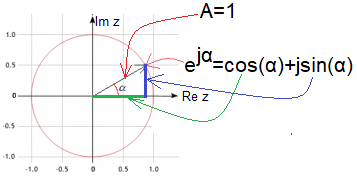
Równanie Eulera
Traktuj kąt α ogólnie jak poczciwe x, tzn. jako liczbę rzeczywistą związaną z równaniem! Zaś jα jest liczbą urojoną na osi Im z. Dopiero z tego równania wynika jego interpretacja z okręgiem i trójkątem prostokątnym. Tu wyraźnie widać, że liczba rzeczywista α jest kątem w radianach. Dla dowolnej rzeczywistej liczby α wartość zespolona z=exp(jα) będzie leżała gdzieś na okręgu o promieniu A=1. W pierwszej chwili wydaje się to tak oczywiste, jak definicje sinusa i cosinusa. Ale jaki związek ma zespolona funkcja wykładnicza exp(jα) z trygonometrią? Pan Euler w swoich czasach mógł korzystać tylko z zespolonego dodawania, odejmowania, mnożenia i dzielenia . A co z funkcją zespoloną exp(jω0t)? Jak ją obliczyć korzystając tylko z podstawowych czterech działań? Euler już jednak wiedział, że rzeczywista funkcja exp(x) jest sumą nieskończenie wielu zmniejszających się wielomianów, tak jak np. liczba 1 to nieskończona suma szeregu 1/2+1/4+1/8+1/16+… Analogicznie potraktował zespoloną funkcję wykładniczą exp(jx). Tzn. obliczył jej wartość jako sumę wielomianów korzystając tylko z czterech działań na liczbach zespolonych. I chyba zdziwił się, gdy punkt z=exp(jx) zaczął wirować po okręgu o promieniu A=1. Dopiero wtedy skojarzył x z kątem α. A spodziewał się, że funkcja będzie dążyć gdzieś do nieskończoności. Tak jak rzeczywista funkcji wykładniczych exp(x) dla x>0! Podstaw do wzoru Eulera kolejno α=0, 0.25π, 0.5π, 0.75π …2π. Zobaczysz jak punkt z=exp(jα) wiruje po okręgu.
Rozdział 2.3 Obsługa video
Główną zaletą artykułu jest animacja. O wiele bardziej działa na wyobraźnię niż zwykły wykres.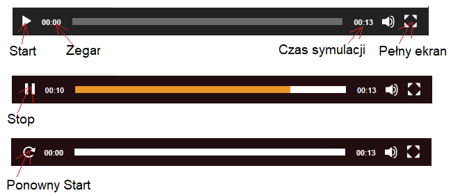
Rys. 2-2
Opis przyciski i wskaźników video
-Start kliknięcie uruchamia animację i zmienia się w przycisk Stop
-Zegar aktualny czas eksperymentu, także jako żółty pasek
-Czas symulacji inaczej-czas trwania eksperymentu, tu 13 sek.
-Pełny ekran kliknięcie powiększa ekran, ponowne kliknięcie zmniejsza itd…
-Stop Kliknięcie zatrzymuje symulację i zmienia się w przycisk Ponowny Start
-Ponowny Start jak sama nazwa wskazuje.
Rozdział 2.4 Badanie różnych ruchów harmonicznych f(t) jako dwuwymiarowych F(jω0t)
Rozdział jest tylko pretekstem do zapoznania się z funkcją zespoloną Start*exp(jω0t). Podkreślam, że parametry Start i jω0t są liczbami zespolonymi! Znając już obsługę video, zbadamy ruchy harmoniczne dla różnych stanów początkowych wirującego wektora Start i pulsacji ω0. Przekonasz się, że funkcja czasu x(t) jest rzutem wirującego wektora Start*exp(jω0t) na oś rzeczywistą Re z. Czyli x(t)=Re z {Start*exp(jω0t)}.
Zbadamy 5 ruchów harmonicznych.
1. 1cos(1t) jako Start*exp(jω0t) dla Start=1 i ω0=1/sek
2. 1sin(1t) jako Start*exp(jω0t) dla Start=1*exp(-jπ/2)=1*exp(-j90°)=-1j i ω0=1/sek,
3. 1cos(1t-π/4) jako Start*exp(jω0t) dla Start=1*exp(-jπ/4)=1*exp(-j45°)≈0.707-j0.707 i ω0=1/sek
4. 1cos(2t) jako Start*exp(jω0t) dla Start=1 i ω0=2/sek
5. 0.5cos(1t) jako Start*exp(jω0t) dla Start=0.5 i ω0=1/sek
Rozdział 2.4.1 f(t)=1*cos(1t) jako F(jω0t)=1*exp(j1t) czyli jako Start*exp(jω0t) dla Start=1 oraz ω0=1/sek
Najważniejszy wniosek:
Wirujący wektor F(jω0t)=1*exp(j1t) jest dwuwymiarową wersją funkcji f(t)= x(t)=1*cos(1t). Tu ω0=1/sek.
Później okaże się, że prawie każda dowolna funkcja okresowa f(t) o okresie T odpowiadającym pulsacji ω=2π/T ma swoją dwuwymiarową wersję jako suma F(jt)=c1*exp(j1ω0t)+c2*exp(j2ω0t)+c3*exp(j3ω0t)…
c1, c2, c3…,cn są to liczby zespolone albo wektory an+jbn jako stany początkowe wirujących wektorów cn*exp(jnω0t).
W dwuwymiarowej wersji F(jω0t) funkcji f(t) niektóre cechy są bardziej widoczne i intuicyjne niż w jednowymiarowej.
Rys. 2-3
Rys. 2-3a
x(t)=1cos(1t)
Jest to ruch jednowymiarowy, bo tylko wzdłuż osi rzeczywistej Re z na płaszczyźnie zespolonej Re z, Im z. Kliknij przycisk “Start” lub rysunek aby zobaczyć 2 okresy T ruchu harmonicznego. Znamy amplitudę A=1 i czas 2 okresów, czyli 2T≈12 sek≈12.56 sek≈4πsek pokazany na stoperze video,
czyli T=2πsek–>ω0=2/T=1/sek. Wartości bezwzględne prędkości są największe w środku, a najmniejsze czyli zerowe na krańcach “przy zawrotkach”.
Rys. 2-3b
Funkcja zespolona 1exp(jω0t) jako wirujący wektor o długości 1 i stanie początkowym (1,0)
Uwaga:
Ponieważ punkt Start=z=(1,0)=1+0j
To funkcja zespolona ma wartość Start*exp(j1t)= (1+0j)*exp(j1t)=1*exp(j1t) i jest nią wirujący wektor o długości 1 i stanie początkowym (1,0).
Dobrze widać, że animacja z Rys. 2-3a jest rzutem animacji z Rys. 2-3b na oś rzeczywistą Re z
Lub inaczej
“Część rzeczywista funkcji zespolonej 1exp(j1t) jest funkcją 1cos(1t).
Lub jeszcze inaczej
Re 1exp(j1t)=1cos(1t)
Rzut obracającego się wektora na oś rzeczywistą Re z, porusza się tak, jak na Rys. 2-3a.
Niektórzy prawie utożsamiają exp(jω0t) z cos(ω0t). Nie jest to ścisłe, ale za to celne i obrazowe. Tak jak sławne zdanie “Jestem za, a nawet przeciw”. Wiemy o co chodzi, choć z logiką na bakier.
Stan początkowy krążącego wektora Start=(1+0j)=+1 widzisz na Rys. 2-3b przed animacją.
Zapamiętaj. Drugi raz nie będę powtarzał!
Każdy wektor Start jest stanem początkowym i “stoi w miejscu”. Tu Start=z=1+0j, ale może nim być np. Start=z=2-3j.
Po pomnożeniu Startprzez exp(jω0t) wektor Start*exp(jω0t) zacznie wirować z prędkością ω0. Przekonasz się o tym także w następnych animacjach.
Rys. 2-3c
Wykres czasowy x(t)=1cos(1t) (ω0=1/sek)
-oś pozioma(“x”) to czas t w sekundach.
Punkty charakterystyczne 0sec, 0.5πsec≈1.57sec, πsec≈3,14sec i 0.75πsec≈2.36sec 2πsec≈6,28 sec
-oś pionowa(“y”) to x(t) w jednostkach
Spróbuj zatrzymać symulację “mniej więcej” w tych czasach i porównać Rys. 2-3a, Rys. 2-3b i Rys. 2-3c.
Rozdział 2.4.2 f(t)=1*sin(1t) jako F(jt)=Start*exp(jω0t) dla Start=-1j oraz ω0=1/sek
Rys. 2-4
Rys. 2-4a
x(t)=x(t)=1sin(1t)
Jest to rzut krążącego wektora z Rys. 2-4b na oś rzeczywistą Re z.
Rys. 2-4b
Funkcja zespolona –1j*exp(j1t) dla ω0=1/sec, inaczej exp(j1t-π/2)*exp(j1t) bo –1j=exp(j1t-π/2)
Uwaga:
Ponieważ punkt Start=0-1j=-1j
To funkcja zespolona ma wartość Start*exp(j1t)=-1j*exp(j1t).
Stan początkowy krążącego wektora Start=-1j widzisz na Rys. 2-4b przed symulacją.
Porównaj z Rys. 2-3b. Dobrze widać, że sin(ω0t) jest opóźniony o π/2 =90º względem cos(ω0t).
Rys. 2-4c
Wykres czasowy x(t)=1sin(1t)
Rozdział 2.4.3 f(t)=1*cos(1t-π/4) jako F(jt)=Start*exp(jω0t) dla Start=1*exp(-jπ/4)=0.707-j0.707 oraz ω0=1/sek
Rys. 2-5
Rys. 2-5a
x(t)=1cos(1t-π/4) czyli x(t)=Acos(ω0t-ϕ) dla A=1 ω0=1/sek i ϕ=π/4 =45º
Jest to rzut krążącego wektora z Rys. 2-4b na oś rzeczywistą Re z.
Rys. 2-5b
Funkcja zespolona 1*exp(j1t-π/4) jako 1*cos(1t-π/4).
Zauważ, że pięknie tu widać opóźnienie ϕ=-π/4 (ϕ=-45º). Sprawdź pitagorasem, że amplituda A=1 oraz, że ϕ=-π/4 =-45º.
Krążący wektor możemy zapisać różnymi sposobami.
Start*exp(j1t)=exp(-jπ/4)*exp(j1t)=(1/√2-j1/√2)*exp(j1t)≈(0.707-j0.707)*exp(j1t).
Stan początkowy krążącego wektora Start=exp(-jπ/4) widzisz na Rys. 2-5b .
Rys. 2-5c
Wykres czasowy x(t)=1cos(1t-π/4)
Rozdział 2.4.4 f(t)=1*cos(2t) jako F(jt)=Start*exp(jω0t) dla Start=1 i ω0=2/sek
Zwiększyliśmy prędkość do ω0=2/sek wzgl. Rys. 2-3
Rys. 2-6
Rys. 2-6a
Przebieg 2 razy szybszy niż na Rys. 2-3. Poza tym stan początkowy Start taki sam czyliStart=(1+0j)=+1
Porównaj z odpowiednimi animacjami z Rys. 2-3.
x(t)=1cos(2t).
Rys. 2-6b
Funkcja zespolona 1exp(j2t) jako 1cos(2t)
Uwaga:
Rys. 2-6c
Wykres czasowy x(t)=1cos(2t)
Rozdział 2.4.5 f(t)=0.5cos(1t) jako F(jω0t)=Start*exp(jω0t) dla Start=0.5 i ω0=1/sek
Rys. 2-7
2 razy mniejsza amplituda A=0.5 porównaj z Rys. 2-4!
Rys. 2-7a
x(t)=0.5cos(1t).
Rys. 2-7b
Funkcja zespolona 0.5exp(j1t) jako 0.5cos(1t)
Rys. 2-7c
Wykres czasowy x(t)=0.5cos(1t).
Rozdział 2.5 Funkcje Start*exp(jω0t)
Porównaj jeszcze raz wcześniej omówione funkcje zespolone dla różnych parametrów Start i ω0.
1- Start=1 i ω0=1/sek
2- Start=1*exp(-jπ/2)=-j1 i ω0=1/sek
3- Start=1*exp(-jπ/4) i ω0=1/sek
4- Start=1 i ω0=2/sek
5- Start=0.5 i ω0=1/sek
Rys. 2-8
5 wersji Start*exp(jω0t)
Funkcje te były przedstawione na Rys.2-4b…Rys.2-7b jako wirujące wektory. Ich końce wskazują punkty z, których współrzędne są właśnie funkcjami zespolonymi Start*exp(j ω0t).
“Buraczkowy“ wektor to stan początkowy każdej funkcji. Jest to parametr Start występujący przed exp(jω0t). Przeanalizuj dokładnie każdy z 5 przebiegów, uwzględniając parametry Start i ω.
Porównaj np. Rys. 2-8b i Rys. 2-8a. Tu lepiej niż na wykresach czasowych widać, że sin(1t)–>-j1exp(j1t) jest opóźniony o 90° względem cos(1t)–>1exp(j1t).
Rozdział 2.6 Funkcja F(jt)=(a-jb)*exp(jω0t) jako dwuwymiarowa wersja f(t)=a*cos(ω0t)+b*sin( ω0t)
Rozdział 2.6.1 Opis ogólny
Deser na koniec. Czyli jak zbudować trajektorię F(jω0t) dla dowolnej funkcji sinusoidalnej f(t)=a*cos(ω0t)+b*sin(ω0t)=c*cos(ω0t-ϕ)
Z Rozdziału 2.4.1 wiemy, że funkcji zespolonej 1*exp(jω0t) odpowiada przebieg czasowy 1*cos(ω0t).
Analogicznie wg. Rozdziału 2.4.2 funkcji zespolonej -1j*exp(jω0t) odpowiada 1*sin(ω0t).
Zapiszemy to tak :
1*exp(jω0t)<==>1*cos(ω0t)
–1j*exp(jω0t)<==>1*sin(ω0t)
Tak jest gdy mamy do czynienia z amplitudami a=1 dla cosinusa i b=1 dla sinusa.
Działa to dla dowolnych amplitud a i b:
a*exp(jω0t)<==>a*cos(ω0t)
-jb*exp(jω0t)<==>b*sin(ω0t)
Zamiast pisać, że funkcji coś tam odpowiada, można bardziej ściśle, tak jak jak poniżej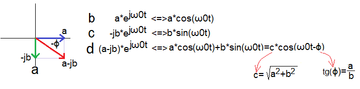
Rys. 2-9
Re (a-jb)*exp(jω0t)=a*cos(ω0t)+b*sin(ω0t)
Wektor (a-jb) wiruje z prędkością ω.
Rzut wirującego wektora (a-jb)*exp(jω0t) na oś rzeczywistą to:
część rzeczywista (a-jb)*exp(jω0t)
czyli Re (a-jb)*exp(jω0t)=a*cos(ω0t)+b*sin(ω0t).
Jest to uogólnienie najprostszego przypadku z Rys.2-3 gdzie a=1 i b=0.
Rys. 2-9a
Funkcja zespolona (a-jb)*exp(jω0t) jako wirujący z prędkością ω0 wektor (a-jb)
Ma ona 2 składowe:
-rzeczywistą (cosinus) a*exp(jω0t)
-urojoną (sinus) -jb*exp(jω0t)
To co widzisz na Rys. 2-9a, jest stanem początkowym wirującego wektora, czyli dla t=0.
Podkreślam, że “samotne” a i b to liczby rzeczywiste!
Rys. 2-9b
Rzut wirującego a*exp(jω0t) wektora na oś rzeczywistą to a*cos(ω0t)
Rys. 2-9c
Rzut wirującego -jb*exp(jω0t) wektora na oś urojoną to b*sin(ω0t)
Rys. 2-9d
Rzut sumy wirujących wektorów, czyli czerwonego wektora na oś rzeczywistą to a*cos(ω0t)+b*sin(ω0t)=c*cos(ω0t-ϕ)
Nie jest to bardzo oczywiste, ale taka jest trygonometria! Zamiast dowodu*, podstawmy konkretne
wartości np. a=0.75 i b=1.25 i sprawdźmy animację.
*Może to zrobić uczeń liceum klasy matematycznej.
Rozdział 2.6.2 Konkretny przykład F(jω0t)=(0.75-j1.25)*exp(jω0t) jako dwuwymiarowa wersja f(t)=0.75*cos(ω0t)+1.25*sin(ω0t)
Rys. 2-10
Wirujący wektor (0.75-j1.25)*exp(1jt) jako f(t)=0.75*cos(1t)+1.25*sin(1t)=1.458*cos(1t-59.04°)
Rys. 2-10a
Wirujący wektor 0.75*exp(1jt) i jego rzut na oś Re z jako funkcja czasu 0.75*cos(1t)
Rys. 2-10b
Wirujący wektor -j1.25*exp(1jt) i jego rzut na oś Re z jako funkcja czasu 1.25*sin(1t)
Rys. 2-10c
Suma 2 lewych wektorów jako wirujący wektor (0.75-j1.25)*exp(1jt)
Jego rzut na oś Re z jest funkcją czasu f(t)=0.75*cos(1t)+1.25*sin(1t)=1.458*cos(1t-59.04°) i jego wykres czasowy przedstawiony jest na poniższej animacji.
Rys. 2-11
1.458*cos(1t-59.04°)=0.75*cos(1t)+1.25*sin(1t)
Przesunięcie kątowe 59.04° ≈1.03 radiana widoczne jest na wykresie.