Wirujące Szeregi Fouriera
Rozdział 11. Sprawdzenie wzorów na Szereg Fouriera programem Wolfram Alfa
Rozdział 11.1 Wstęp
Moim głównym celem jest przekonanie Czytelnika do poniższych wzorów dokładnie omówionych w rozdz. 7.2. Nie są łatwe, ale mam nadzieję, że duża ilość przykładów z animacjami pomogła nieco. Wiadomo, że środek ciężkości scn trajektorii dla danej prędkości obrotowej nω0, to już prawie n-ta harmoniczna. Wzór Rys. 11-1b na ogół zgadza się z intuicją, zwłaszcza dla scn=(0,0) gdy harmonicznej dla nω0 nie ma. Właśnie, zgadzał się z intuicją, ale nie był obliczany. Teraz skorzystamy z programu WolframaAlfa z internetu. Nic nie musisz instalować, ani płacić. Przy okazji się z nim zapoznasz. Szkoda, że jako student w latach 60-tych nie mogłem z niego korzystać.

Rys. 11-1
Wzory do zapamiętania z rozdz. 7.
Sprawdzimy je programem WolframAlfa. Potem będą bardziej zjadliwe.
Rys. 11-1a
Trajektoria F(njω0t)
Punkt porusza się na osi rzeczywistej Re Z zgodnie z funkcją okresową f(t) a płaszczyzna Z wiruje z ω=-nω0. W ten sposób rysowana jest trajektoria F(njω0t).
Rys. 11-1b
Wzór na środek ciężkości scn trajektorii F(njω0t).
Funkcją podcałkową jest trajektoria F(njω0t). Całkę (podzieloną przez T) możemy traktować jako punkt scn średnio odległy trajektorii F(njω0t) od początku współrzędnych (0,0) w czasie T sek. Tak jak Ziemia krąży wokół Słońca, tak trajektoria F(njω0t) krąży wokół “środka ciężkości” scn.
Rys. 11-1c
Wzór na składową stałą c0=a0 szeregu Fouriera. Klasyczna średnia funkcji okresowej f(t), gdy n=0 we wzorze Rys. 11-1b.
Rys. 11-1d
Wzór na na pozostałe n-te współczynniki szeregu Fouriera cn dla ω=1ω0, ω=2ω0…ω=nω0.
Inaczej, n-ta amplituda zespolona harmonicznej hn(t)
Rys. 11-1e
cn jako wektor (liczba zespolona) o składowych an oraz jbn
Rys. 11-1f
cn w wersji wersji algebraicznej
cn=an-jbn
Rys. 11-1g.
cn w wersji wersji wykładniczej
cn=|cn|*exp(-jϕn)
Wyraźnie widać moduł |cn| i fazę ϕn dla pulsacji ω=nω0.
Rys. 11-1h
n-ta harmoniczna hn(t) jako suma składowej cosinusoidalnej i sinusoidalnej.
Rys. 11-1i
n-ta harmoniczna hn(t) jako cosinus z przesunięciem fazowym ϕ
Moduł |cn|, inaczej moduł |cn| jest “pitagorasem” z an i bn, zaś tg(ϕ)=bn/an.
Rozdział 11.2 Program WolframaAlfa
Sprawdzimy nim wzory na środki cięzkości scn poznanych trajektorii. Większość tego typu programów ma jedną wadę. Aby rozwiązać problem, musisz go ściśle zdefiniować. Pomylisz się w postawieniu kropki i już pojawia się “error” lub inny trudny do zrozumienia komunikat. WolframAlfa jest taki mądry, że wystarczy mu zadać pytanie ogólne, a on poda wiele odpowiedzi. Tym więcej, im bardziej ogólne było pytanie. Wybierzesz tę odpowiedź, która Ci najbardziej pasuje. Dzięki temu nie musisz się pamiętać wszystkich instrukcji WolframAlfa i możesz całkowicie skupić się na problemie.
Chcemy np. rozwiązać równanie 2x+3=7.
1. Należy wywołać program z internetu.
2. Wpisać do okienka 2x+7=3.
3. Program nie bardzo wie, o co Ci chodzi. Na wszelki wypadek narysuje wykres i poda rozwiązanie x=–2. Tobie zależało na tym ostatnim.
Uwaga:
Po wywołaniu programu wyjdziesz z tego bloga. Aby do niego powrócić, kliknij windowsową strzałkę powrotu –>.
Kliknij https://wolframalpha.com i rób co każe poniższy obrazek.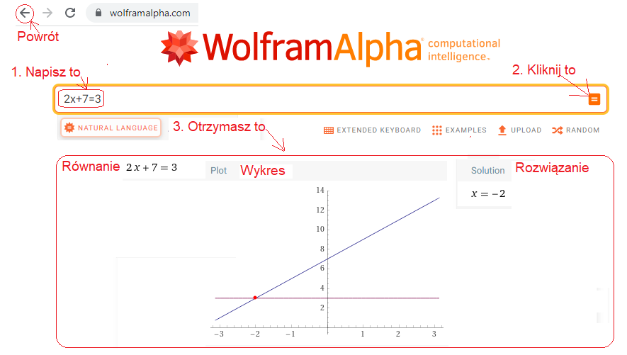
Rys. 11-2
Jak WolframAlfa rozwiązał równanie 2x+7=3?
Dla Ciebie najważniejsze jest rozwiązanie–> solution x=–2. A wykres jako dodatkowa odpowiedź nie zaszkodzi.
To był elementarz. Ciekawe, jak WolframAlfa poradzi sobie z całkowaniem? Zwłaszcza z całkowaniem wektorów albo liczb zespolonych.
Obliczmy teraz środki ciężkości i przy okazji n-te harmoniczne dla kliku poznanych funkcji okresowych f(t). Wcześniej musiałeś przyjąć środki ciężkości scn na wiarę. Teraz je obliczysz.
Rozdział 11.3 Środek ciężkości sc1 trajektorii F(jnω0t)=F(-1j1t)=1*exp(-1j1t)
Rozdział 11.3.1 Wstęp
Czyli dla funkcji stałej f(t)=1. z p. 7.4.1 rozdz.7. Jest to funkcja okresowa, bo co okres T funkcja się powtarza. Mało tego, co dowolny okres T!
Rys. 11-3
Funkcja zespolona 1exp(-1j1t) jako trajektoria i jej “środek ciężkości” sc.
Rys. 11-3a
Funkcja zespolona 1exp(-1j1t) jako wirujący wektor.
Kliknij. W ciągu okresu T=2π/ω≈6.28sek wektor wykona jeden obrót. A gdybyśmy w czasie obrotu sumowali kolejne wektory?
Rys. 11-3b
Okrąg jako ślad po wirującym wektorze czyli trajektoria 1exp(-1j1t).
Rys.11-3c
Wzór na środek ciężkości scn trajektorii funkcji. Gdy np. n=1 to wzór Rys.11-3c (1/2π)*exp(-1jω0t) dla ω0=-1/sek.
Już bez obliczeń widać, że środkiem ciężkości jest sc1=(0,0). Czy wzór Rys.11-1b to potwierdzi?
Rozdział 11.3.2 WolframAlfa
Obliczmy środek ciężkości sc1 trajektorii F(-1j1t)=f(t)*exp(-1j1t).
Kliknij https://wolframalpha.com i rób co każe obrazek.
Zamiast pracowicie wpisywać instrukcję, możesz ją po prostu skopiować
integrate 1*exp(-i1t)/(2pi) from t=0 to t=2pi
i wkleić do okienka.
Innymi słowy, do okienka wkleisz wzór całkowy Rys. 11-1b zapisany w języku WolframAlfa. Pamiętaj, że liczbą urojoną dla WolframAlfa jest “matematyczne i“, a nie “elektryczne j” używane w blogu.
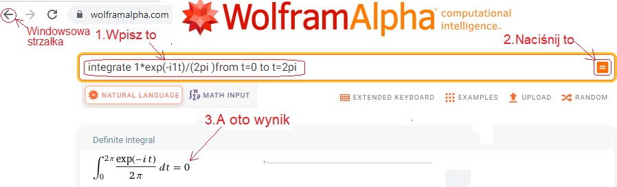
Rys. 11-4
Środek ciężkości sc1=(0,0) trajektorii F(-1j1t)=1exp(-1j1t)
Tak jak się spodziewaliśmy, środek ciężkości sc1=0 a ściślej sc1=(0,0), bo jest to liczba zespolona. Miły jest ten Wolframik. Np. Instrukcję z okienka zamienia na ludzki, czyli matematyczny język. Widać to przy strzałce “3. A oto wynik”.
Powracając do wyniku sc1=0, to co z niego wynika? A no to, że amplituda pierwszej harmonicznej c1 dla harmonicznej 1ω0=1/sek jest zerowa, bo cn=2*sn. Czyli nie ma harmonicznej o pulsacji ω=1/sek, ani także dla każdej innej pulsacji ω. Tego się spodziewaliśmy i jedyną składową funkcji stałej f(t)=1 jest składowa stała c0=1.
Rozdział 11.4 Środki ciężkości scn trajektorii F(-njω0t)=0.5cos(4t)*exp(-njω0t) dla n=0, 1, 4 i ω0=1/sek
Rozdział 11.4.1 Wstęp
Jest to skrócona wersja rozdziału 4, w którym było 9 wersji tej trajektorii dla n=0…9. Teraz są tylko 3 wersje dla n=0,1 i tylko tylko te wzory sprawdzimy rachunkowo.
Wrzućmy do wirówki funkcję f(t)=0.5cos(4t).
Włączmy obroty na n=0, n=1 i n=4. Czyli na prędkość ω=0 (wirówka stoi!), ω=-1/sek i ω=-4/sek.
Powstaną 3 trajektorie:
n=0–>ω=0–>wirówka stoi–>F(-0j1t)=0.5cos(4t)
n=1–>ω=-1/sek –>F(-1j1t)=0.5cos(4t)*exp(-1j1t)
n=4–>ω=-4/sek –>F(-4j1t)=0.5cos(4t)*exp(-4j1t)
Rys. 11-5
Trzy trajektorie F(-nj1t)=0.5cos(4t)*exp(nj1t) dla n=0, 1 i 4
ω=0
Wirówka stoi, bo ω=0 i sc0=(0,0)
ω=-1/sek
Wirowanie ω=-1/sek i sc1=(0,0)
ω=-4/sek
Wirowanie ω=-4/sek i sc4=(0.25,0)
Powyższe parametry sc0, sc1 i sc0,, choć intuicyjne, były przyjęte na “słowo honoru”. Teraz obliczymy je programem WolframAlfa. Wyniki powinny być takie same.
Rozdział 11.4.2 Środek ciężkości sc0, czyli dla ω=0, czyli składowa stała sc0=c0=a0.
Czyli gdy wirówka stoi, bo n=0
Wtedy trajektoria F(-0j1t)=f(t)=0.5cos(4t)
Z animacji Rys. 11-4a ω=0 wynika, że trajektorią jest bujająca się w poziomie linia wg. funkcji f(t)=0.5cos(4t). Jej środkiem ciężkości jest ewidentnie sc0=(0,0). Czy WolframAlfa to potwierdzi? Wstawmy f(t)=0.5cos(4t) do wzoru Rys. 11-1c i obliczmy tą całkę.
Kliknij https://wolframalpha.com i rób co każe obrazek.
Do okienka wpisz lub wklej integrate 0.5cos(4t)/(2pi) from t=0 to t=2pi
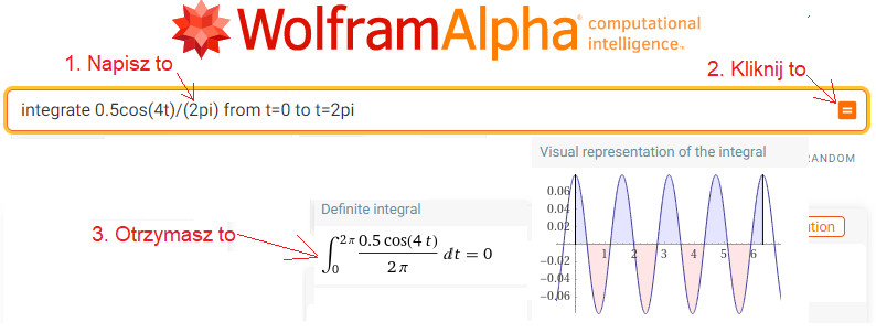
Rys. 11-6
Obliczenie środka ciężkości sc0 dla F(0j1t)=0.5cos(4t)*exp(-0j1t)=0.5cos(4t)
sc0=0
Zauważ, że chociaż okresem podstawowym f(t) jest T=π/2,to wynik sc0=0 dla granic całkowania T=π/2 i T=2π będzie taki sam!
Granice całkowania we wzorze Rys. 11-1c mogą być dowolne i wynik będzie taki sam dla np. T=0.234 sek, T=5.27 sek czy T=2π sek jak w powyższym wzorze! Ważne tylko, żeby T było okresem funkcji. Uwaga ta jest bardziej ogólna i dotyczy wzorów na Szereg Fouriera we wzorze Rys. 11-1b. Jedni podają dowolne granice całkowania T, a inni tak jak ja, konkretne T=2π. Współczynniki Fouriera np. fali prostokątnej nie zależą przecież od okresu T, tylko od kształtu tej fali!. Środek ciężkości sc0 dla trajektorii każdej funkcji f(t) jest jednocześnie składową stałą tej funkcji i jest współczynnikiem c0=a0 szeregu Fouriera. W odróżnieniu od pozostałych współczynników Fouriera tj. c1, c2…cn, współczynnik c0 jest zawsze liczbą rzeczywistą.
Rozdział 11.4.3 Środek ciężkości sc1, czyli dla ω=-1/sek.
Czyli sc1 trajektorii F(-1j1t)=0.5cos(4t)*exp(-1j1t) z Rys.11-5 ω=-1/sek
Szukamy harmonicznej o pulsacji ω=1/sek z funkcji f(t)=0.5cos(4t). Oczywiste jest, że nie istnieje. Przecież jedyną harmoniczną f(t) jest ona sama, czyli 0.5cos(4t). Wynika to także z Rys. 11-4 ω=-1/sek, w którym sc1=(0,0). Czy WolframAlfa to potwierdzi?
Kliknij https://wolframalpha.com i rób co każe obrazek.
Do okienka wpisz lub wklej integrate [0.5cos(4t)/(2pi)]*exp(-1i1t) from t=0 to t=2pi
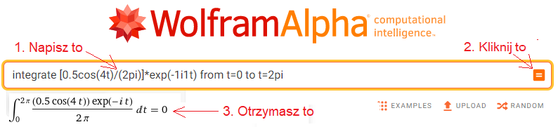
Rys. 11-7
Środek ciężkości sc1=0 trajektorii 0.5cos(4t)*exp(-1j1t)
Amplituda c1=0 dla harmonicznej ω=1/sek bo c1=2sc1=0. Czyli nie ma takiej harmonicznej.
Jak się przekonałeś w Rozdziale 4, środki ciężkości dla wszystkich ω różnych od 4/sek (czyli od ω funkcji 0.5cos(ωt)) są zerowe. Jest to jak, mówił klasyk, oczywista oczywistość. Przecież funkcja 0.5cos(4t) ma tylko jedną harmoniczną i jest nią ona sama! Pozostałe harmoniczne są zerowe.
Rozdział 11.4.4 Środek ciężkości sc4, czyli dla ω=-4/sek.
Czyli sc4 trajektorii F(-4j1t)=0.5cos(4t)*exp(-4j1t) z Rys.11-4 ω=-4/sek
Szukamy harmonicznej o pulsacji ω=4/sek z funkcji f(t)=0.5cos(4t). Chyba każdy widzi tą harmoniczną. Jest nią ona sama 0.5cos(4t).
Funkcja f(t)=0.5cos(4t) obraca się zegarowo z prędkością ω=-4/sek. Zauważ, że f(t) i wirówka mają takie ω=4/sek (choć przeciwne znaki)! Spowodowało to przesunięcie środka ciężkości z sc=(0,0) na sc4=(+0.25,0).
Aby sprawdzić rachunkowo kliknij https://wolframalpha.com i rób co każe obrazek.
Do okienka wpisz lub wklej integrate [0.5cos(4t)]*exp(-i4t)/(2pi) from t=0 to t=2pi.
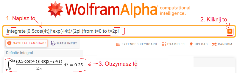
Rys. 11-8
Środek ciężkości sc4=0.25 a ściślej sc4=(0.25,0) trajektorii 0.5cos(4t)*exp(-4j1t)
Okaże się, że dla każdej prędkości wirowania ω funkcji 0.5cos(4t)/(2pi) różnej od ω=4/sek środek ciężkości scn=(0,0), a tylko dla ω=4/sek jest niezerowe sc4=(+0.25,0)!
Wg. wzoru Rys. 11-1d
c4=2*sc4=(+0.5,0) czyli a4=0.5 i b4=0
Wg. wzoru Rys. 11-1h
h4(t)=0.5cos(4t).
Rozdział 11.5 Środki ciężkości scn trajektorii F(-njω0t)=[1.3+0.7*cos(2t)+0.5*cos(4t)]*exp(-njω0t)
czyli F(-njω0t) dla n=0,2,3,4 i ω0=1/sek
Rozdział 11.5.1 Wstęp
Jest to skrócona wersja rozdziału 5, w którym było 9 trajektorii dla n=0…9. Teraz będą tylko 4 dla n=0,2,3 i 4.
Wrzućmy do wirówki funkcję f(t)=1.3+0.7*cos(2t)+0.5*cos(4t)
Włączmy obroty na ω=0, ω=-2/sek, ω=-3/sek, i ω=-4/sek.
Powstaną 4 trajektorie:
n=0–>ω=0–>wirówka stoi–>F(0j1t)=1.3+0.7*cos(2t)+0.5*cos(4t)
n=1–>ω=-2/sek –>F(-1j1t)=[1.3+0.7*cos(2t)+0.5*cos(4t)]*exp(-2j1t)
n=3–>ω=-3/sek –>F(-3j1t)=[1.3+0.7*cos(2t)+0.5*cos(4t)]*exp(-3j1t)
n=4–>ω=-4/sek –>F(-4j1t)=[1.3+0.7*cos(2t)+0.5*cos(4t)]*exp(-4j1t)
Rys. 11-9
Cztery trajektorie F(-nj1t)=[1.3+0.7*cos(2t)+0.5*cos(4t)]*exp(-nj1t) dla n=0, 1, 2 i 4 i ich środki ciężkości scn.
Pokazano przebiegi w czasie jednego okresu T=2π sek odpowiadającemu pulsacji pierwszej harmonicznej a1cos*cos(1t), dla której a1=0. Czyli nie ma jej w f(t). Przebiegi ω=-2/sek i ω=-4/sek “rysowane są na sobie” i dlatego pozornie zatrzymały się po 1π sek.
ω=0
Wirówka stoi i sc0=(1.3,0)
ω=-2/sek
Wirowanie ω=-2/sek i sc2=(0.35,0)
ω=-3/sek
Wirowanie ω=-3/sek i sc3=(0,0)
ω=-4/sek
Wirowanie ω=-4/sek i sc4=(0.5,0)
Środki ciężkości scn są w miarę intuicyjne, ale w rozdziale 5 były ujęte bez uzasadnienia.
Teraz obliczymy je wg. wzoru Rys. 1-11b programem WolframAlfa. Wyniki powinny być takie same.
Rozdział 11.5.2 Środek ciężkości sc0 dla ω=0.
Czyli sc0 trajektorii F(-0j1t)=[1.3+0.7*cos(2t)+0.5*cos(4t)] z Rys.11-9 ω=0. Wirówka stoi. Trajektorią jest koniec bujającej się w poziomie linii wg. funkcji F(-0j1t)=f(t)=1.3+0.7*cos(2t)+0.5*cos(4t). Jej środkiem ciężkości jest sc0=(1.3,0)=1.3.
Obliczmy sc0=c0=a0 czyli składową stałą wg Rys. 1-11c.
Kliknij https://wolframalpha.com i rób co każe obrazek.
Do okienka wpisz lub wklej instrukcję WolframAlfa dla w.w całki , czyli integrate [1.3+0.7*cos(2t)+0.5*cos(4t)]/(2pi) from t=0 to t=2pi
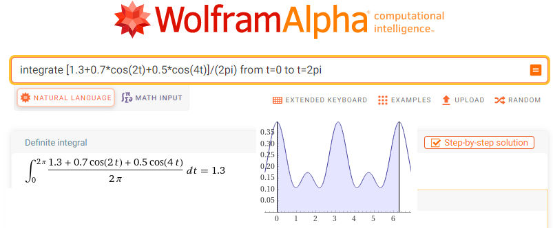
Rys. 11-10
Obliczenie środka ciężkości sc0 dla F(0j1t)=[1.3+0.7*cos(2t)+0.5*cos(4t)]/(2pi)
Środek ciężkości sc0=(1.3,0)=1.3 dla niewirującej trajektorii funkcji f(t) jest jej składową stałą, czyli współczynnikiem c0=a0 szeregu Fouriera.
Rozdział 11.5.3 Środek ciężkości sc2 dla ω=2/sek.
Czyli sc2 trajektorii F(-2j1t)=[1.3+0.7*cos(2t)+0.5*cos(4t)]*exp(-2j1t) dla z Rys.11-9 ω=-2/sek
Kliknij https://wolframalpha.com.
Do okienka wpisz lub wklej integrate [1.3+0.7*cos(2t)+0.5*cos(4t)]*exp(-2i1t)]/(2pi) from t=0 to t=2pi
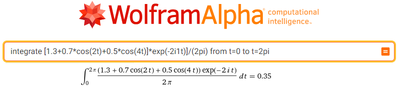
Rys. 11-11
Obliczenie środka ciężkości sc2 dla F(2j1t)=[1.3+0.7*cos(2t)+0.5*cos(4t)]*exp(-2j1t)/(2pi)
Środek ciężkości sc2=(0.35,0)=0.35, czyli amplituda drugiej harmonicznej to c2=2*(0.35,0]=(0.7,0).czyli a2=0.7 b2=0
Druga harmoniczna to h2(t)=0.7*cos(2t) wg. wzoru Rys. 11-1e.
Rozdział 11.5.4 Środek ciężkości sc3 dla ω=3/sek.
Czyli sc3 trajektorii F(-3j1t)=[1.3+0.7*cos(2t)+0.5*cos(4t)]*exp(-3j1t) z Rys.11-9 ω=-3/sek.
Kliknij https://wolframalpha.com i rób co każe obrazek.
Do okienka wpisz lub wklej integrate [1.3+0.7*cos(2t)+0.5*cos(4t)]*exp(-3j1t) from t=0 to t=2pi
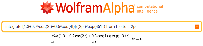
Rys. 11-12
Obliczenie środdka ciężkości sc3 trajektorii [1.3+0.7*cos(2t)+0.5*cos(4t)]*exp(-3j1t)/(2pi)
Środek ciężkości sc3=(0,0)=0, czyli amplituda trzeciej harmoniczna c3=2*0=0
Trzecia harmoniczna nie istnieje. Nie istnieje także 5,6,7… harmoniczna. Widać to oczywiście w samej funkcji f(t), ale możesz sprawdzić to programem WolframAlfa.
Rozdział 11.5.5 Środek ciężkości sc4 dla ω=4/sek.
Czyli sc4 trajektoriii F(-4j1t)=[1.3+0.7*cos(2t)+0.5*cos(4t)]*exp(-4j1t) dla Rys.11-9 ω=-4
Kliknij https://wolframalpha.com.
Do okienka wpisz lub wklej integrate [1.3+0.7*cos(2t)+0.5*cos(4t)]*exp(-4i1t)]/(2pi) from t=0 to t=2pi
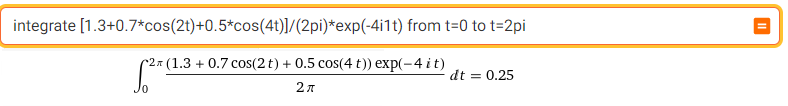
Rys. 11-13
Obliczenie środka ciężkości sc4 dla F(4j1t)=[1.3+0.7*cos(2t)+0.5*cos(4t)]*exp(-4j1t)/(2pi)
Środek ciężkości sc4=(0.25,0)=0.25, czyli amplituda czwartej harmoniczna c4=2*0.25=0.5 a4=0.5 b4=0
Czwarta harmoniczna to h4(t)=0.5*cos(4t) wg. wzoru Rys. 1-11h.
Rozdział 11.6 Środki ciężkości scn trajektorii f(4j1t)=0.5cos(4t-30°)*exp(-4j1t) dla ω=4/sek
czyli z całkowicie zespolonym środkiem ciężkości scn
Do tej pory środki ciężkości scn harmonicznych z funkcji f(t) były liczbami rzeczywistymi np. Rys. 11-9 ω=–2/sek –->sc2=(+0.35,0)=+0.35. Są to także liczby zespolone, ale z zerowymi składowymi urojonymi. A co będzie gdy funkcja cosinus będzie miała przesunięcie fazowe.
Wrzućmy więc do wirówki np. f(t)=0.5cos(4t-30°).
Włączmy obroty na n=0, n=1 i n=4.
Powstaną 3 trajektorie:
n=0–>ω=0–>wirówka stoi–>F(-0j1t)=0.5cos(4t-30°)
n=1–>ω=-1/sek –>F(-1j1t)=0.5cos(4t-30°)*exp(-1j1t)
n=4–>ω=-4/sek –>F(-4j1t)=0.5cos(4t-30°)*exp(-4j1t)
Rys. 11-14
F(4j1t)=0.5cos(4t-30°)*exp(-jnt) dla n=0,1,4
Animacja trwa T≈6.28sek.
ω=0
F(0j1t)=0.5cos(4t-30°)
Różnica między animacją Rys. 11-5 ω=0 jest minimalna, ale spróbuj ją zauważyć.
ω=-1/sek.
F(4j1t)=0.5cos(4t-30°)*exp(-j1t)
Trajektoria obrócona jest o (podejrzewam) -30° względem Rys. 11-5 ω=-1/sek. Środek ciężkości sc=(0,0).
Oznacza to, że nie istnieje harmoniczna funkcji f(t)=0.5cos(4t) dla ω=1/sek. Także dla każdej innej, oprócz ω=4/sek.
ω=-4/sek.
F(4j1t)=0.5cos(4t-30°)*exp(-j4t)
Trajektoria obrócona jest o ϕ=-30° względem Rys. 11-5 ω=-4/sek.
Środek ciężkości sc5 jest pełną gębą liczbą zespoloną sc4=(a,b) gdzie:
a=0.25cos(-30°)≈+0.217
b=0.25sin(-30°)≈-0.125
sc=(a,b)≈(+0.217,-0.125)=+0.217-j0.125
Czyli zespolona czwarta harmoniczna h4(t)≈2*sc≈2*(+0.217-j0.125)*exp(j4t). Odpowiada ona funkcji f(t)=0.434cos(4t)+0.25sin(4t)=0.5cos(4t-30°) wg. wzorów Rys.11-1 h oraz Rys.11-1 i
Co na to WolframAlfa?
Kliknij https://wolframalpha.com.
Do okienka wpisz lub wklej integrate [0.5cos(4t-pi/6)]/(2pi)*exp(-4i1t) from t=0 to t=2pi
Uwaga -30° to -π/6 w radianach
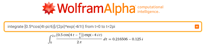
Rys. 11-15
sc4=0.216506-j0.125
Taki środek ciężkości sc4 trajektorii F(4j1t)=0.5cos(4t-30°)*exp(-j4t) policzył WolframAlfa. Wynik podobny do naszego, tylko dokładniejszy. Zwróć uwagę na to że sc4 jest liczbą w pełni zespoloną. Tak jest, gdy wirująca funkcja typu cosinus/sinus ma niezerowe przesunięcie fazowe ϕ. Tu ϕ=-30°=-π/6.
Ciekawostka
Porównaj animacje Rys. 11-13 ω=-1/sek i ω=-4/sek.
ω=-1/sek
Czterolistna koniczynka
ω=-4/sek
To też jest pewnego rodzaju ileśtamlistna koniczynka z tym że:
Każdy listek jest okręgiem i jest rysowany “jeden na drugim”.
Co do “ileśtamlistna”, to podejrzewam, że też czterolistna.
Rozdział 11.7 Środki ciężkości scn trajektorii
F(-njω0t)=[0.5+1.08*cos(1t-33.7°)+0.72*cos(3t+33.7°)+0.45*cos(5t-26.6°)]*exp(-njω0t)
dla n=0,1,2,…8 i ω0=1/sek
Rozdział 11.7 Wstęp
Sama funkcja f(t) o okresie T=2πsek wygląda tak i nie widać w niej składowych, czyli trzech cosinusoid z różnymi fazami ϕ.
Rys. 11-16
f(t)=0.5+1.08*cos(1t-33.7°)+0.72*cos(3t+33.7°)+0.45*cos(5t-26.6°)
W Rozdziale 6 badaliśmy 9 trajektorii F(-njω0t) tej funkcji f(t) dla n=0,1,2,…8 i ω0=1/sek. Jest ona o tyle ciekawa, że ze względu na przesunięcia fazowe ϕ, środki ciężkości scn są liczbami całkowicie zespolonymi. Funkcja f(t) jest równoważna poniższej, w której każda harmoniczna została rozłożona na składową cosinusoidalną i sinusoidalną
f(t)=0.5+0.9*cos(1t)+0.6*sin(1t)+0.6*cos(3t)-0.4*sin(3t)+0.4*cos(5t)+0.2*sin(5t).
Np. 0.9*cos(1t)+0.6*sin(1t)=1.08*cos(1t-33.7°)
Jest to ta sama funkcja, ale tu łatwo wyznacza się zespolone współczynniki Fouriera, inaczej zespolone amplitudy Fouriera.
Z nich odczytuje się harmoniczne jako przebiegi czasowe h1(t),h2(t) i h3(t) o składowych sinus/cosinus.
c1=0.9-j0.6—>h1(t)=0.9*cos(1t)+0.6*sin(1t)
c3=0.6+j0.4–>h3(t)=0.6*cos(3t)-0.4*sin(3t)
c5=0.4-j0.2—>h5(t)=0.4*cos(5t)+0.2*sin(5t)
Uwaga:
Obie postacie funkcji f(t) są równoważne, ale do obliczeń przyjmiemy wersję z “cosinusami i sinusami”
Funkcje f(t) włożymy do wirówki z różnymi prędkościami nω0=-n*1/sek dla n=0,1,2,3 i 5. Sprawdzimy czy obliczone środki ciężkości scn są takie same jak w Rozdziale 6.
Rozdział 11.7.2 Środki ciężkości scn trajektorii F(-njω0t)=f(t)*exp(-njω0t) dla n=0, 1,2, 3, 5 i ω0=1/sek
Wrzućmy do wirówki funkcję z Rys.11-15. Przypominam, że można ją przedstawić też w wersji sinus/cosinus tj: f(t)=0.5+0.9*cos(1t)+0.6*sin(1t)+0.6*cos(3t)-0.4*sin(3t)+0.4*cos(5t)+0.2*sin(5t).
Włączmy obroty na n=0, 1, 2, 3 i 5. Czyli na prędkości ω=0 (wirówka stoi!), ω=-1/sek ,ω=-2/sek, ω=-3/sek i ω=-5/sek.
Powstanie 4 trajektorii:
ω=0–>wirówka stoi–>F(-0j1t)=f(t)
ω=-1/sek –>F(-1j1t)=f(t)*exp(-1j1t)
ω=-2/sek –>F(-2j1t)=f(t)*exp(-2j1t)
ω=-3/sek –>F(-3j1t)=f(t)*exp(-3j1t)
ω=-5/sek –>F(-5j1t)=f(t)*exp(-5j1t)
Rys. 11-17
5 trajektorii F(-nj1t)=f(t)*exp(nj1t) dla n=0,1,2,3 i 5 ω=0 i ich środki ciężkości scn
ω=0
Wirówka i sc0=(+0.5,0)
ω=-1/sek
Wirowanie ω=-1/sek i sc1=(+0.45,-0.3)
ω=-2/sek
Wirowanie ω=-2/sek i sc2=(0,0)
ω=-3/sek
Wirowanie ω=-3/sek i sc3=(+0.3,+0.2)
ω=-5/sek
Wirowanie ω=-5/sek i sc5=(+0.2,-0.1)
Przypominam, że wektor scn to już prawie n-ta harmoniczna okresowej funkcji f(t). Ściślej wektor 2*scn jest zespoloną amplitudą n-tej harmonicznej. W okresie T=2π każdą trajektorię rysuje zmieniający się wektor i scn jest średnią tych zmieniających się wektorów w okresie T=2π, czyli ich sumą podzieloną przez 2π.
Środki ciężkości scn obliczymy programem WolframAlfa. Wyniki powinny być identyczne.
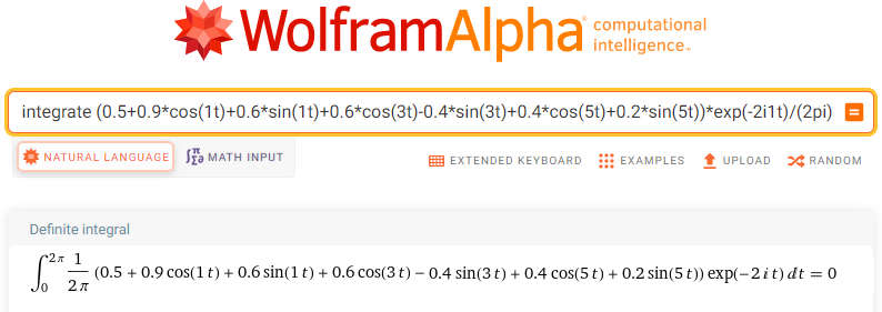
Rozdział 11.7.3 Środek ciężkości sc0, czyli dla ω=0
Trajektoria F(-0j1t)=f(t) z Rys.11-16 ω=0.
Wirówka stoi. Trajektorią jest koniec bujającej się w poziomie linii na Rys.11-16 ω=0 wg. funkcji F(-0j1t)=f(t). Jej środkiem ciężkości jest sc0=(+0.5,0)=+0.5.
Wstawmy f(t) do wzoru Rys. 11-1c.
Do okienka wpisz lub wklej instrukcję WolframAlfa dla w.w całki , czyli
integrate [0.5+0.9*cos(1t)+0.6*sin(1t)+0.6*cos(3t)-0.4*sin(3t)+0.4*cos(5t)+0.2*sin(5t)]/(2pi) dt from t=0 to t=2pi
Kliknij https://wolframalpha.com i rób co każe obrazek.
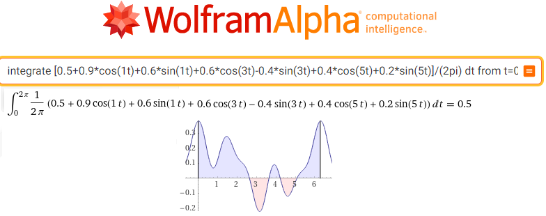
Rys. 11-18
Obliczenie środka ciężkości sc0 dla F(0j1t)=f(t)/(2pi)
Środek ciężkości sc0=(0.5,0)=a0=0.5 dla niewirującej trajektorii funkcji f(t) jest jej składową stałą, czyli współczynnikiem c0=a0 szeregu Fouriera.
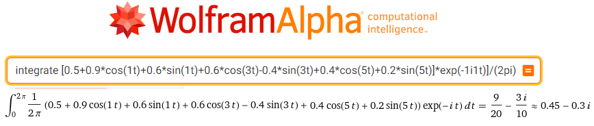
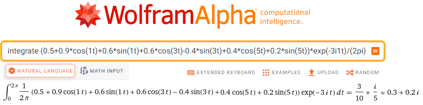
Rozdział 11.7.4 Środek ciężkości sc1 dla ω=1/sek.
Trajektoria F(-1j1t)=f(t)*exp(-1j1t) z Rys.11-16 ω=-1/sek
Do okienka wpisz lub wklej
integrate [0.5+0.9*cos(1t)+0.6*sin(1t)+0.6*cos(3t)-0.4*sin(3t)+0.4*cos(5t)+0.2*sin(5t)]*exp(-1i1t)]/(2pi) dt from t=0 to t=2pi
Kliknij https://wolframalpha.com.
Rys. 11-19
Trajektoria F(-1j1t)=f(t)*exp(-1j1t)
Uwaga:
W okienku widzisz tylko końcówkę wyrażenia które wkleiłeś.
sc1=0.45-j0.3
Zespolona amplituda pierwszej harmonicznej to 2*sc1=0.9-j0.6
Czyli pierwsza harmoniczna wg Rys. 11-1h i Rys. 11-1i to h1(t)=0.9cos(1t)+0.6sin(1t)=1.08*cos(1t-33.7°).
Sukces! WolframAlfa idealnie odfiltrował pierwszą harmoniczną z funkcji okresowej f(t).
Tego samego spodziewamy się w następnych rozdziałach
|
Rozdział 11.7.5 Środek ciężkości sc2 dla ω=2/sek.
Trajektoria F(-2j1t)=f(t)*exp(-2j1t) z Rys.7-18 ω=-2/sek
Do okienka wpisz lub wklej
integrate (0.5+0.9*cos(1t)+0.6*sin(1t)+0.6*cos(3t)-0.4*sin(3t)+0.4*cos(5t)+0.2*sin(5t))*exp(-2i1t)/(2pi) dt from t=0 to t=2pi
Kliknij https://wolframalpha.com.
Rys. 11-20
Trajektoria F(-2j1t)=f(t)*exp(-2j1t)
sc2=0 czyli nie istnieje harmoniczna o pulsacji ω=2/sek
Rozdział 11.7.6 Środek ciężkości sc3 dla ω=3/sek.
Trajektoria F(-3j1t)=f(t)*exp(-3j1t) z Rys.7-18 ω=-3/sek
Do okienka wpisz lub wklej
integrate (0.5+0.9*cos(1t)+0.6*sin(1t)+0.6*cos(3t)-0.4*sin(3t)+0.4*cos(5t)+0.2*sin(5t))*exp(-3i1t)/(2pi) dt from t=0 to t=2pi
Kliknij https://wolframalpha.com.
Rys. 11-21
Trajektoria F(-3j1t)=f(t)*exp(-3j1t)
sc3=0.3+j0.2
Zespolona amplituda trzeciej harmonicznej to 2*sc=0.6+j0.4
czyli trzecia harmoniczna wg Rys. 11-1h i Rys. 11-1i to h3(t)=0.6cos(3t)-0.4sin(3t)≈0.72*cos(3t+33.7°).
Rozdział 11.7.7 Środek ciężkości sc5 dla ω=5/sek.
Trajektoria F(-5j1t)=f(t)*exp(-5j1t) z Rys.11-16 ω=-5/sek
Do okienka wpisz lub wklej
integrate (0.5+0.9*cos(1t)+0.6*sin(1t)+0.6*cos(3t)-0.4*sin(3t)+0.4*cos(5t)+0.2*sin(5t))*exp(-3i1t)/(2pi) dt from t=0 to t=2pi
Kliknij https://wolframalpha.com.
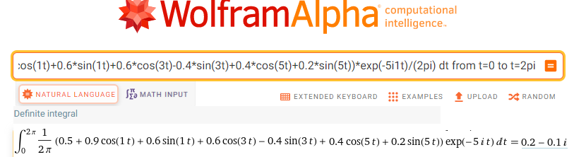
Rys. 11-22
Trajektoria F(-5j1t)=f(t)*exp(-5j1t)
sc=0.2-j0.1
Zespolona amplituda piątej harmonicznej to 2*sc=0.4-j0.2
czyli piąta harmoniczna wg Rys. 11-1h i Rys. 11-1i to h5(t)=0.4cos(5t)+0.2sin(5t)≈0.45*cos(5t-26.6°)
Rozdział 11.7.8 “Środek ciężkości” scn trajektorii F(-njω0t)=f(t)*exp(-njω0t) dla n=4,6,7,8 i ω0=1/sek
Pozostały jeszcze środki ciężkości sc4, sc6, sc7 i sc8 czyli dla n=4, 6, 7 i 8.Są zerowe czyli nie występują harmoniczne dla tych pulsacji n*ω0. Proponuję samemu dokonać obliczeń programem WolframAlfa i sprawdzić czy są takie same jak w Rozdziale 6. Tam też zobaczysz odpowiednie trajektorie.
Rozdział 11.8 Środki ciężkości scn trajektorii fali prostokątnej parzystej dla n=0,1,2,…8 i ω0=1/sek
Rozdział 11.8.1 Wstęp
Powtórzymy rodz.8, ale tym razem obliczymy środki ciężkości trajektorii scn programem WolframAlfa. Poprzednio przyjęliśmy je na wiarę.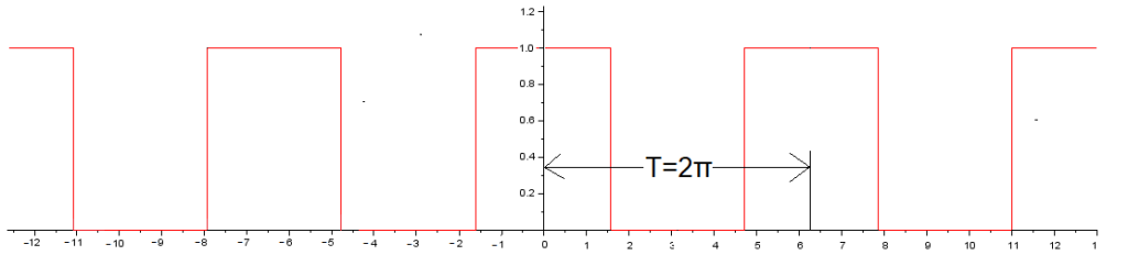
Rys. 11-23
Fala prostokątna parzysta f(t) A=1, ω=1/sek, ϕ=0 i w=50%.
Obliczymy kolejne harmoniczne programem Wolframu Alfa stosując wzory z Rys.11-1. Ale najpierw sprawdzimy jak WolframAlfa radzi sobie z falą prostokątną.
Rozdział 11.8.2 Fala prostokątna f(t) i WolframAlfa
Wiemy jak wygląda instrukcja funkcji np. sin(t) w WolframAlfa. Funkcja sin(t) to po prostu sin(t). Natomiast fala prostokątna to squarewave[t]. Zróbmy wykres tej funkcji instrukcją plot.
Kliknij https://wolframalpha.com.
Do okienka wpisz lub wklej
plot squarewave[t] from t=-2 to 2
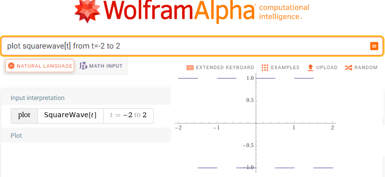
Rys.11-24
Fala prostokątna wywołana funkcją squarewave[t] from t=-2 to 2
Jest to funkcja nieparzysta, okresowa T=1sek, A=2 bez składowej stałej.
Jak ją zmodyfikować, żeby otrzymać falę parzystą z rozdz.8?
Należy
1. Przemnożyć przez 0.5 żeby zmniejszyć amplitudę z A=2 na A=1
2. “Rozciągnąć” z okresu T=1sek do T=2πsek
3. Przesunąć w lewo o π/2sek aby funkcję nieparzystą zmienić na parzystą.
4. Przesunąć w górę o 0.5
Zbadajmy ją,
Kliknij https://wolframalpha.com.
Do okienka wpisz lub wklej
plot 0.5*squarewave[(t+0.5pi)/(2pi)]+0.5 from t=-2π to 2π
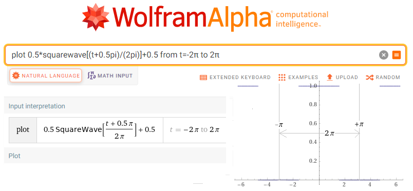
Rys.11-25
Fala prostokątna z Rys.11-23 wywołana programem WolframAlfa.
Pokazano okres T=2π funkcji f(t), ściślej t od –π do +π.
W następnych rozdziałach wyznaczymy jej trajektorie, środki ciężkości scn i harmoniczne hn(t).
Rozdział 11.8.3 Środek ciężkości sc0, czyli dla ω=0, czyli składowa stała a0.
Skorzystamy ze wzoru Rys.11-1c
Kliknij https://wolframalpha.com.
Do okienka wpisz lub wklej
(1/(2pi))*integrate [[0.5+ 0.5*SquareWave[(t+pi/2)/(2pi)]] from t=-pi to t=+pi
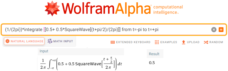
Rys.11-26
Obliczenie składowej stałej sc0=c0=a0=+0.5
Tak jak się spodziewaliśmy, a0=0.5 jako średnia wartość fali prostokątnej w okresie od –π do +π. Nawet nie trzeba było całkować, bo a0 jako średnią widać na Rys.11-23.
Rozdział 11.8.4 Środek ciężkości sc1, czyli dla ω=-1/sek.
Czyli sc1 trajektorii F(-1j1t)=f(t)*exp(-1j1t) gdzie f(t) jest falą prostokątną z Rys.11-23. Powtórzymy animację z Rys. 8-3 rozdz. 8.
Rys.11-27
Trajektoria F(1j1t) fali prostokątnej parzystej
Rys.11-25a
Wektor 1exp(j1j1t) jako promień R=1 wirujący z prędkością ω=-1/sek
Rys.11-25b
Wektor F(1j1t) jako promień R=1 modulowany falą prostokątną f(t) z Rys.11-23.
Rys.11-25c
Trajektoria F(1j1t) fali prostokątnej parzystej rysowana przez koniec wektora z Rys.11-25b
Wektor środka ciężkości trajektorii sc1=(1/π,0) mniej więcej zgadza się z intuicją, Przecież jako średnia obracającego się wektora z Rys.11-25b musi leżeć gdzieś pomiędzy (0,0) a (1,0). Policzmy go teraz dokładnie programem WolframAlfa.
Skorzystamy ze wzoru Rys.11-1c
Kliknij https://wolframalpha.com.
Do okienka wpisz lub wklej
[(1/(2pi)]*integrate [[0.5+ 0.5*SquareWave[(t+pi/2)/(2pi)]]*exp(-1i1t)dt from t=0 to t=+2pi
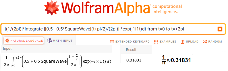
Rys.11-28
Obliczenie sc1=(1/π,0)
Program obliczył średnią z wektorów w czasie T=2πsek i wyszło mu 0.31831.
Po pierwsze to policzył dokładniejszą wartość ale zaokrąglił do 5 cyfr po przecinku.
Po drugie jest to dokładnie liczba 1/π
Po trzecie jest to wektor w postaci liczby zespolonej sc1=(1/π,0)
Rozdział 11.8.5 Środek ciężkości sc2=0, czyli dla ω=-2/sek.
Czyli sc2 trajektorii F(-2j1t)=f(t)*exp(-1j1t) gdzie f(t) jest falą prostokątną z Rys.11-23. Powtórzymy animację z Rys. 8-5 rozdz. 8.
Rys.11-29
Trajektoria F(2j1t) fali prostokątnej parzystej
Rys.11-29a
Wektor 1exp(j2j1t) jako promień R=1 wirujący z prędkością ω=-2/sek
Rys.11-29b
Wektor F(2j1t) jako promień R=1 modulowany falą prostokątną f(t) z Rys.11-23.
Rys.11-29c
Trajektoria F(2j1t) fali prostokątnej parzystej rysowana przez koniec wektora z Rys.11-27b
Wektor środka ciężkości trajektorii sc2=(0,0) zgadza się z intuicją jako średnia. Policzmy go teraz dokładnie programem WolframAlfa.
Skorzystamy ze wzoru Rys.11-1c
Kliknij https://wolframalpha.com.
Do okienka wpisz lub wklej
[(1/(2pi)]*integrate [[0.5+ 0.5*SquareWave[(t+pi/2)/(2pi)]]*exp(-2i1t)dt from t=0 to t=+2pi
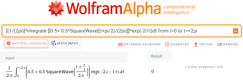
Rys. 11-30
Obliczenie sc2=0=(0,0)
Czyli druga harmoniczna, ściślej dla ω=2/sek nie występuje.
Rozdział 11.8.6 Środek ciężkości sc3, czyli dla ω=-3/sek.
Czyli sc3 trajektorii F(-3j1t)=f(t)*exp(-3j1t) gdzie f(t) jest falą prostokątną z Rys.11-23. Powtórzymy animację z Rys. 8-6 rozdz. 8.
Rys.11-31
Trajektoria F(1j1t) fali prostokątnej parzystej
Rys.11-31a
Wektor 1exp(j1j1t) jako promień R=1 wirujący z prędkością ω=-1/sek
Rys.11-31b
Wektor F(1j1t) jako promień R=1 modulowany falą prostokątną f(t) z Rys.11-23.
Rys.11-31c
Trajektoria F(3j1t) fali prostokątnej parzystej rysowana przez koniec wektora z Rys.11-31b
Wektor środka ciężkości trajektorii sc3=(-1/3π,0). Do interpretacji najlepiej nadaje się animacja Rys.11-31b. Zauważ, że wektor wykonuje 2 x 3/4 obrotu. Lewy kierunek wektora na osi Rez jest oczywisty, gdy uwzględnimy 2 puste ćwierćobroty. Gdyby ich nie było (2x1 obrót), to sc3=(0,0). A dlaczego długość wektora sc3 jest mniejsza od długości sc1 na Rys.11-27c? Bo więcej jest przerw w okresie T=2πsek, co zmniejsza średnią. Ostatecznie przekona Cię WolframAlfa.
Skorzystamy ze wzoru Rys.11-1c
Kliknij https://wolframalpha.com.
Do okienka wpisz lub wklej
[(1/(2pi)]*integrate [[0.5+ 0.5*SquareWave[(t+pi/2)/(2pi)]]*exp(-3i1t)dt from t=0 to t=+2pi
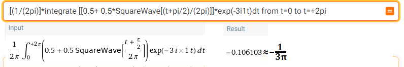
Rys.1-32
Obliczenie sc3=(-1/3π,0)
Rozdział 11.8.7 Środek ciężkości sc4=0, czyli dla ω=-4/sek.
Czyli sc4 trajektorii F(-4j1t)=f(t)*exp(-4j1t) gdzie f(t) jest falą prostokątną z Rys.11-23. Powtórzymy animację z Rys. 8-6 rozdz. 8.
Rys.11-33
Trajektoria F(4j1t) fali prostokątnej parzystej
Rys.11-33a
Wektor 1exp(4j1t) jako promień R=1 wirujący z prędkością ω=-4/sek
Rys.11-33b
Wektor F(4j1t) jako promień R=1 modulowany falą prostokątną f(t) z Rys.11-23.
Rys.11-33c
Trajektoria F(4j1t) fali prostokątnej parzystej rysowana przez koniec wektora z Rys.11-33b
Wektor środka ciężkości trajektorii sc4=(0,0) zgadza się z intuicją jako średnia. Policzmy go teraz programem WolframAlfa.
Skorzystamy ze wzoru Rys.11-1c
Kliknij https://wolframalpha.com.
Do okienka wpisz lub wklej
[(1/(2pi)]*integrate [[0.5+ 0.5*SquareWave[(t+pi/2)/(2pi)]]*exp(-4i1t)dt from t=0 to t=+2pi
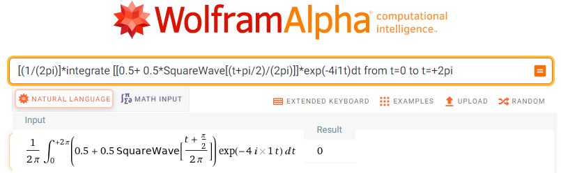
Rys. 11-34
Obliczenie sc4=(0,0)
Rozdział 11.8.8 Środki ciężkości sc5,sc6,sc7 i sc8, czyli dla ω=-5/sek, -6/sek,-7/sek i- 8/sek.
Jako praca domowa. Podpowiem tylko, że wystarczy do Wolframowego okna wkleić
[(1/(2pi)]*integrate [[0.5+ 0.5*SquareWave[(t+pi/2)/(2pi)]]*exp(-ni1t)dt from t=0 to t=+2pi
z odpowiednio zmienionym n.