Rotating Fourier Series

Chapter 3 Summation of rotating vectors exp(jωt)

Chapter 3.1 What’s that for?
To make it easier to understand the summation of the cos(ωt) function, more broadly – sinusoidal type functions.
And how he found it fits Fourier Series, which is the sum of sines and cosines.

Chapter 3.2 General summation of rotating vectors exp(jωt)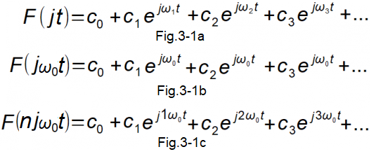


Fig.3-1
Fig.3-1a
Sum of rotating vectors F(jt) where:
c0 is a constant component or, in other words, a rotating vector with a speed ω=0
c1, c2, c3… is a complex number that is the initial state of each spinning vector c1*exp(jω1t), c2exp(jω2t),ec3xp(jω3t)…
ω1, ω2, ω3… The pulsations of ω1, ω2, ω3… are arbitrary! i.e. may or may not be multiples of the first harmonic ω1. This is the most general sum formula and we will not analyze this case.
Fig.3-1b
Sum of rotating F(jnω0t) vectors with the same ω0 pulsation.
It is a complex number vector c=c1+c2+c3+… rotating at a speed of ω0.
The real number c0 is a constant component.
The sum of sine and cosine is also a sine with the same pulsation ω0 and the corresponding phase shift φ.
It is used in classical electrical engineering, where power plants generate electricity with a constant frequency f=50Hz, i.e. ω0=314*1/sec. The topic has already been thoroughly worked out, probably in the 19th century.
Example with animation in chapter 3.3
Fig.3-1c
This is what we’ll mainly be dealing with.
i.e. sum of rotating vectors F(njω0t) with increasing pulsations 1ω0,2ω0, 3ω0…
I emphasize that each pulsation is a multiple of the basic pulsation ω0, and not any ω1, ω2, ω3 … as in Fig. 3-1a
Examples with animation in chapters 3.4…7

Chapter 3.3 Sum of 2 rotating vectors exp(jωt) with the same pulsation ω0=1/sec i.e. 1*exp(j1t)-j1exp(j1t)
The case of Fig.3-1b when c0=0, c1=1, c2=1*exp(-jπ/2)=-j1 and c3=c1+c2=1-j1=√2*exp(-jπ/4 )
The numbers c1, c2 and c3 are the initial states of the rotating vectors as in Fig.3-2 before the animation.
Notice that the vector c2 is lagging behind by π/2=90º with respect to c1.

Fig. 3-2
Sum of 2 rotating vectors as:
1exp(j1t)-j1*exp(j1t) or (1-1j)exp(j1t) or √2exp(-jπ/4)*exp(j1t) where -π/4=-45º. The right vector is at any time the sum of the 2 left vectors and has parameters A=√2, ω=1/sec and ϕ=-π/4=-45º. At the initial moment, i.e. before pressing “Start”, the sum, i.e. the right vector, agrees (vectorically add the left vectors–>”diagonal of the square”). Then pause the simulation at any time by clicking on the drawing or “Start” and check if it is correct.
The most important conclusion.
When all vectors have the same rotational speed ω0, then their sum is also a rotating vector with the same speed ω0, length A which is constant and phase ϕ.
Note1
Applies to any number of rotating vectors.
Note2
Notice that the relative position of all 3 rotating vectors is constant! This makes it very easy to analyze e.g. electrical circuits. When this is not the case, e.g. Fig. 3-1a or 3-1c, and the vectors rotate at different speeds, the sum vector changes length and speed! You will find out in Chapter 3.4.

Chapter 3.4 Sum F(njω0t)=1exp(j1t)+1exp(j2t)
Chapter 3.4.1 “Vector Only” Version
We begin to study sums of rotating vectors with different pulsations. “Vector only” means that the ends of the vectors do not draw a trajectory.
The case of Fig.3-1c when c0=0 c1=1, c2=1 and ω0=1/sec

Fig. 3-3
F(jω0t)=1*exp(1jt)+1*exp(2jt) (ω0=1/sec)
You see vector functions as rotating vectors
1*exp(1jt), 1*exp(2jt) and their sum 1*exp(1jt)+1*exp(2jt)
You can clearly see 2 times the speed of 1*exp(2jt). Try to stop the animation at different times t and check if the right function is a vector sum of the left 2. Here 

Chapter 3.4.2 Trajectory or “Trace only” version
“Trace only” means that the ends of the vectors draw a trace. The vectors themselves are invisible and this trace is the trajectory F(jω0t). This is the case of Fig.3-1c when c0=0 c1=1, c2=1 and ω0=1/sec. Only one animation period is shown. Further rotations follow the same paths and the animation looks static! Also in the next animations.
Here and further we will limit ourselves to the “only with a trace” version. The “vector” version of this case is the animation in Fig 3-3.

Fig. 3-4
F(njω0t)=1*exp(1jt)+1*exp(2jt)
The right animation is the sum of the 2 left ones. Note that 1*exp(2jt) “stopped” after the first half-period. But the trajectory continues to rotate, only along the same path!

Chapter 3.5  F(njω0t)= 1exp(j1t)+0.7exp(j2t)

Fig. 3-5
F(jω0t)=1exp(j1t)+0.7exp(j2t)

Chapter 3.6 F(njω0t)=1exp(j1t)+1exp(j2t-π/6)

Fig. 3-6
F(jω0t)=1exp(j1t)+1exp(j2t-π/6)
φ= -π/6 is a decent delay φ=-30º.
The previous examples had a phase shift φ=0º, now one of the components 1exp(j2t-π/6) has φ non-zero. The “delaying” component 1exp(j2t-π/6) causes the trajectory to rotate to the left.

Chapter 3.7 F(njω0t)=0.3exp(j1t)+0.5exp(j2t-π/6)+0.45exp(j2t+π/4)
A more complicated trajectory.

Fig. 3-7
F(njω0t)=0.3exp(j1t)+0.5exp(j2t-π/6)+0.45exp(j2t+π/4)
Recall that the sum vector keeps rotating, even after the animation ends after the first period T. The formula in Fig. 3-7 describes the trajectory for ω0=1/sec. The shape of the trajectory will be exactly the same for ω0=2/sec, ω0=3/sec… Except that it will rotate 2, 3… times faster.
The red point in (0,0) is also the so-called center of gravity of the trajectory. More on this in the next chapter.

Chapter 3.8 Conclusions

Fig. 3-8
F(njω0t) as a sum of rotating vectors in which:
– c0 is a constant component or formally a rotating vector with ω=0 pulsation. Is a real number (and complex at the same time!)
– c1exp(1jω0) is a rotating vector with a speed of 1ω0
– c2exp(2jω0) is a rotating vector with a speed of 2ω0
– c3exp(3jω0) is a rotating vector with speed 3ω0
…
And the complex numbers c1, c2, c3… are the initial states of these rotating vectors.
Some treat the initial state as the beginning of the world, and others as the moment t=0, when we start the experiment. Read->press animation. Take a quick look at Fig. 4-8 in the next section. There are coefficients c0=-0.5, c1=0.9-j0.6, c2=0.6+j0.4 and c3=0.4-j0.2 for a particular Fourier Series. The trajectory F(njω0t) is drawn every period T along the same path. This period corresponds to the first harmonic here 1ω0=1/sec and T≈6.28sec.