Rotating Fourier Series

Chapter 11. Checking the Fourier Series formulas with the Wolfram Alfa program

Chapter 11.1 Introduction
My main goal is to convince the reader of the following formulas, thoroughly discussed in chapter. 7.2. They are not easy, but I hope that the large number of examples with animations helped a bit. It is known that the centroid scn of the trajectory for a given rotational speed nω0 is almost the n-th harmonic. The formula of Fig. 11-1b generally agrees with intuition, especially for scn=(0,0) when there is no harmonic for nω0. That’s right, it matched the intuition, but it wasn’t calculated. Now we will use the WolframAlfa program from the Internet. You don’t have to install anything or pay anything. You’ll get to know it along the way. It’s a pity that I couldn’t use it as a student in the 1960s.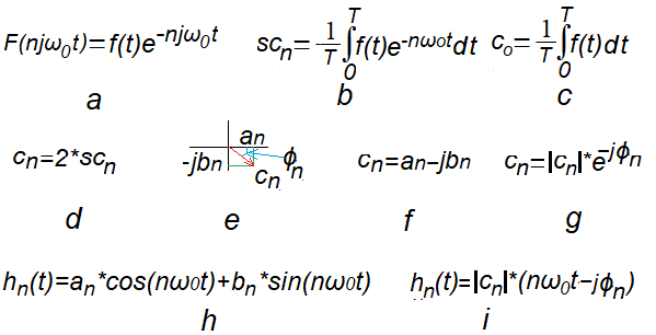

Fig. 11-1
Formulas to remember from chapter 7.
We will check them with the WolframAlfa program. Then they will become more intuitive.
Fig. 11-1a
Trajectory F(njω0t)
The point moves on the real axis Re Z according to the periodic function f(t) and the Z plane rotates with
ω=-nω0. In this way, the trajectory F(njω0t) is drawn.
Fig. 11-1b
Formula for the centroid scn of the trajectory F(njω0t).
The integrand function is the trajectory F(njω0t). We can treat the integral (divided by T) as a point scn that is on average distant in the trajectory F(njω0t) from the point (0,0) in time T sec. Just as the Earth revolves around the Sun, the trajectory F(njω0t) revolves around the centroid scn.
Fig. 11-1c
Formula for the constant component c0=a0 of the Fourier Series. The classical average of the periodic function f(t) when n=0 in the formula Fig. 11-1b.
Fig. 11-1d
The formula for the remaining nth coefficients of the Fourier Series cn for ω=1ω0, ω=2ω0…ω=nω0.
In other words, the nth complex amplitude of the harmonic hn(t)
Fig. 11-1e
cn as a vector (complex number) with components an and jbn
Fig. 11-1f
cn as a algebraic version
cn=an-jbn
Fig. 11-1g.
cn as a exponential version
cn=|cn|*exp(-jϕn)
The |cn| module and phase ϕn is clearly visible for pulsation ω=nω0.
Fig. 11-1h
nth harmonic hn(t) as the sum of the cosine and sinusoidal components.
Fig. 11-1i
nth harmonic hn(t) as cosine with phase shift ϕ
Module |cn|, is a “Pythagoras” of an and bn, and tan(ϕ)=bn/an.

Chapter 11.2 WolframAlfa Program
We will use it to check the formulas for the centroids of the known trajectories. Most of these types of programs have one drawback. To solve a problem, you must define it precisely. If you make a mistake in placing a dot, an “error” or other message that is difficult to understand appears. WolframAlfa is so smart that just ask him a general question and he will give you many answers. Even more so, the more general the question was. You will choose the answer that suits you best. Thanks to this, you do not have to remember all WolframAlfa instructions and you can completely focus on the problem.
For example, we want to solve the equation 2x+3=7.
1. Download the program from the Internet.
2. Enter 2x+7=3 in the box.
3. The program doesn’t really know what you mean. Just to be on the safe side, he will draw a graph and give the solution x=-2. You cared about the latter.
Note:
Once you invoke the WolframAlfa, you will exit this blog. To return to it, click the windows return arrow –>.
Click on https://www.wolframalpha.com and do what the image below tells you to do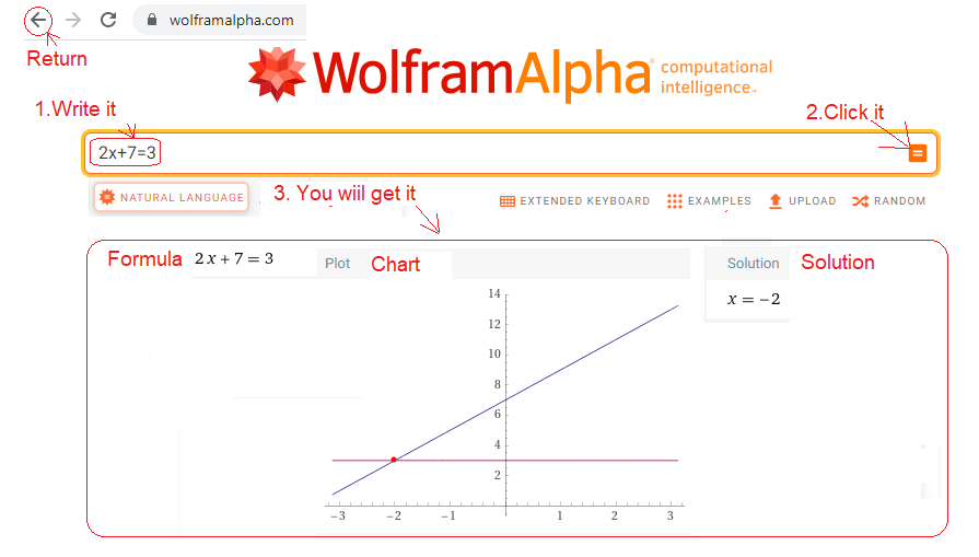

Fig. 11-2
How did WolframAlfa solve the equation 2x+7=3?
The most important thing for you is the solution x=–2. And a time  chart as an additional answer wouldn’t hurt. It was a primer. I wonder how WolframAlfa will handle integration? Especially with integrating vectors or complex numbers. Let us now calculate the centroids and the nth harmonics for several known periodic functions f(t). Previously you had to take the centroids  exact values on faith. Now you will calculate them.

Chapter 11.3 Centroid sc1 of the trajectory F(jnω0t)=F(-1j1t)=1*exp(-1j1t)
Chapter 11.3.1 Introduction
That is, for a constant function f(t)=1. from chapter. 7.4.1. It is a periodic function because the function repeats itself every period T. What’s more, any T period!

Fig. 11-3
Complex function 1exp(-1j1t) as a trajectory and its centroid sc1.
Fig. 11-3a
Complex function 1exp(-1j1t) as a rotating vector.
Click. During the period T=2π/ω≈6.28sec the vector will make one revolution. What if we summed up subsequent vectors during rotation?
Fig. 11-3b
A circle as a trace of a rotating vector, i.e. a trajectory of 1exp(-1j1t).
Fig.11-3c
Formula for the centroid scn of a function trajectory. When, for example, n=1, the formula Fig. 11-3c (1/2π)*exp(-1jω0t) for ω0=-1/sec.
Without any calculations, you can see that the centroid is sc1=(0,0). Will the formula in Fig.11-1b confirm this?
Chapter 11.3.2  Checking with the WolframAlfa
Let us calculate the centroid sc1 of the trajectory https://www.wolframalpha.com and do what the picture says. Instead of laboriously typing instructions, you can simply copy them
integrate 1*exp(-i1t)/(2pi) from t=0 to t=2pi and paste into the window.
In other words, you will paste the integral formula Fig. 11-1b written in the WolframAlpha language into the window. Please note that the imaginary number for WolframAlfa is the “mathematical i”, not the “electrical j” used in the blog.

Fig. 11-4
Centroid sc1=(0,0) trajectory F(-1j1t)=1exp(-1j1t)
As we expected, the centroid sc1=0, or more precisely, sc1=(0,0), because it is a complex number. This WolframAlfa is nice. For example, the instruction from the window is converted into human, i.e. mathematical, language. This can be seen with the arrow “3. You will get it.”
Coming back to the result of sc1=0, what does it mean? Well, the amplitude of the first harmonic c1 for the harmonic 1ω0=1/sec is zero, because cn=2*sn. So there is no harmonic with pulsation ω=1/sec, nor for any other pulsation ω. This is what we expected and the only component of the constant function f(t)=1 is the constant component c0=1.

Chapter 11.4 Centroids scn of trajectories F(-njω0t)=0.5cos(4t)*exp(-njω0t) for n=0, 1, 4 and ω0=1/sec
Chapter 11.4.1 Introduction
This is a shortened version of Chapter 4, which had 9 versions of this trajectory for n=0…9. Now there are only 3 versions for n=0.1 and only these formulas will we check for calculations.
Let’s throw the function f(t)=0.5cos(4t) into a centrifuge.
Let’s turn on the rotations to n=0, n=1 and n=4. So at a speed of ω=0 (the centrifuge is stationary!), ω=-1/sec and ω=-4/sec.
There will be 3 trajectories:
n=0–>ω=0–->centrifuge standing–>F(-0j1t)=0.5cos(4t)
n=1–>ω=-1/sec –->centrifuge rotating–>F(-1j1t)=0.5cos(4t)*exp(-1j1t)
n=4–>ω=-4/sec –->centrifuge rotating–>F(-4j1t)=0.5cos(4t)*exp(-4j1t)

Fig. 11-5
Three trajectories F(-nj1t)=0.5cos(4t)*exp(nj1t) for n=0, 1 and 4
ω=0
The centrifuge is standing because ω=0 and sc0=(0,0)
ω=-1/sec
Centrifugation ω=-1/sec and sc1=(0,0)
ω=-4/sec
Centrifugation ω=-4/sec and sc4=(0.25,0)
The above parameters sc0, sc1 and sc0, although intuitive, were taken on my word of honor. Now we will calculate them with the WolframAlfa program. The results should be the same.
Chapter 11.4.2 Centroid sc0, i.e. for ω=0, i.e. the constant component sc0=c0=a0.
That is, when the centrifuge is standing, because n=0
Then the trajectory F(-0j1t)=f(t)=0.5cos(4t)
The animation Fig. 11-4a ω=0 shows that the trajectory is a horizontally swinging line according to. function f(t)=0.5cos(4t). Its centroid is clearly sc0=(0,0). Will WolframAlfa confirm this? Let’s put f(t)=0.5cos(4t) into the formula Fig. 11-1c and calculate this integral.
Click on https://www.wolframalpha.com and do whatever the picture tells you to do.
In the box, type or paste integrate 0.5cos(4t)/(2pi) from t=0 to t=2pi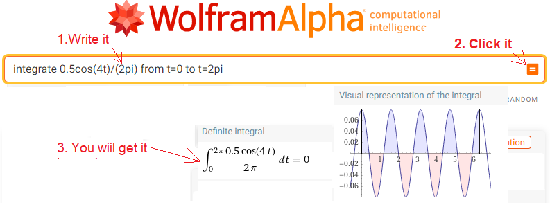

Fig. 11-6
Calculation of the centroid sc0 for F(0j1t)=0.5cos(4t)*exp(-0j1t)=0.5cos(4t)
sc0=0
Note that although the fundamental period of f(t) is T=π/2, the result of sc0=0 for the integration limits of T=π/2 and T=2π will be the same!
The integration limits in the formula Fig. 11-1c can be arbitrary and the result will be the same for e.g. T = 0.234 sec, T = 5.27 sec or T=2π sec as in the above formula! The only important thing is that T is the period of the function. This note is more general and applies to the Fourier Series formulas in Fig. 11-1b. Some give arbitrary limits of integration T, and others, like me, specify specific T=2π sec. The Fourier coefficients of, for example, a square wave do not depend on the period T, but on the shape of the wave! The centroid sc0 for the trajectory of each function f(t) is also the constant component of this function and is the coefficient c0=a0 of the Fourier Series. Unlike the other Fourier coefficients i.e. c1, c2…cn, the coefficient c0 is always a real numbe

Chapter 11.4.3 Centroid sc1, i.e. for ω=-1/sec.
That is, sc1 of the trajectory F(-1j1t)=0.5cos(4t)*exp(-1j1t) from Fig. 11-5 ω=-1/sec. We are looking for a harmonic with pulsation ω=1/sec from the function f(t)=0.5cos(4t). It is obvious that it does not exist. After all, the only harmonic of f(t) is itself, i.e. 0.5cos(4t). This also follows from Fig. 11-4 ω=-1/sec, where sc1=(0,0). Will WolframAlfa confirm this?
Click on https://www.wolframalpha.com and do whatever the picture tells you to do.
In the box, type or paste integrate [0.5cos(4t)/(2pi)]*exp(-1i1t) from t=0 to t=2pi

Fig.11-7
Centroid sc1=0 trajectory 0.5cos(4t)*exp(-1j1t)
Amplitude c1=0 for harmonic ω=1/sec because c1=2sc1=0. So there is no such harmonic.
As you saw in Chapter 4, the centroid for all ω different from 4/sec (that is, from ω of the function 0.5cos(ωt)) are zero. It is obvious. After all, the 0.5cos(4t) function has only one harmonic, and that is itself! The remaining harmonics are zero.

Chapter 11.4.4 Centroid sc4, i.e. for ω=-4/sec.
That is, sc4 of the trajectory F(-4j1t)=0.5cos(4t)*exp(-4j1t) from Fig. 11-4 ω=-4/sec
We are looking for a harmonic with pulsation ω=4/sec from the function f(t)=0.5cos(4t). I guess everyone sees this harmonic. It is itself 0.5cos(4t).
The function f(t)=0.5cos(4t) rotates clockwise at a speed of ω=-4/sec. Note that f(t) and the centrifuge have ω=4/sec (though opposite signs)! This caused the centroid to shift from sc4=(0,0) to sc4=(+0.25,0).
To check the calculation, click https://www.wolframalpha.com and do what the picture tells you.
In the box, enter or paste integrate [0.5cos(4t)]*exp(-i4t)/(2pi) from t=0 to t=2pi.

Fig. 11-8
Centroid sc4 or more precisely sc4=(0.25,0) of the trajectory 0.5cos(4t)*exp(-4j1t). It will turn out that for each spin speed ω of the function 0.5cos (4t)/(2pi) different from ω=4/sec the center of gravity scn=(0,0), and only for ω=4/sec there is a non-zero sc4=(+ 0.25.0)!
Acc. to Fig. 11-1d  c4=2sc4=(+ 0.5,0) that is a4=0.5 and b4=0
Acc. to  Fig. 11-1h  h4(t)=0.5cos (4t).

Chapter 11.5 Centroids scn of trajectories F (-njω0t) = [1.3+0.7cos(2t)+0.5cos (4t)] exp (-njω0t)
that is F (-njω0t) for n = 0,2,3,4 and ω0=1/sec
Chapter 11.5.1 Introduction
It is an abbreviated version of Chapter 5, in which there were 9 trajectories for n = 0… 9. Now there will only be 4 for n=0,2,3 and 4.
Let’s put the function f (t)=1.3+0.7cos (2t)+0.5cos (4t) into the centrifuge
Let the rotation be at ω=0, ω=-2 sec, ω=-3/sec, and ω=-4/sec.
4 trajectories will be created:
n=0–>ω=0–> centrifuge is standing–>F(0j1t)=1.3+0.7cos(2t)+0.5cos (4t)
n=1–>ω=-2/sec–> centrifuge is rotating–> F(-1j1t)=[1.3+0.7cos(2t)+0.5cos(4t)]exp (-2j1t)
n=3–>ω=-3/sec –> centrifuge is rotating–>  F(-3j1t)=[1.3+0.7cos(2t)+0.5cos(4t)]exp(-3j1t)
n=4–>ω=-4/sec–> centrifuge is rotating–> F(-4j1t)=[1.3+0.7cos(2t)+0.5cos(4t)]exp (-4j1t)

Fig. 11-9
Four trajectories F(-nj1t)=[1.3+0.7cos (2t)+0.5cos(4t)]exp(-nj1t) for n=0, 1, 2 and 4 and their centroids scn.
The waveforms during one period T=2π sec. The waveforms ω=-2/sec and ω=-4/sec are “drawn on top of each other” and therefore seemingly stopped after 1π sec.
ω=0 The centrifuge is standing–> sc0=(1.3,0)
ω=-2/sec The centrifuge is rotating–>sc2=(0.35.0)
ω=-3/sec  The centrifuge is rotating–>sc3=(0,0)
ω=-4/sec The centrifuge is rotating –>sc4=(0.5,0)
The centroidsy scn are fairly intuitive, but were included in Chapter 5 without justification. Now we will calculate them by of the formula Fig. 11-1b with the WolframAlfa program. The results should be the same.
Chapter 11.5.2 Centroid sc0 for ω=0
So sc0 of the trajectory F(-0j1t)=[1.3+0.7cos (2t)+0.5cos (4t)] from Fig. 11-9 ω = 0. The centrifuge is standing. The trajectory is the horizontally swinging line acc. to F(-0j1t)=f (t)= 1.3+ 0.7cos (2t)+0.5cos(4t). Its centroid is sc0=1.3=(1.3,0).
Let us calculate sc0=c0=a0 that is the constant component acc. to Fig. 1-11c.
Click on https://www.wolframalpha.com and do what the picture tells you to do.
Enter or paste the WolframAlfa instruction for the integral, i.e.
integrate[1.3+0.7*cos (2t)+0.5*cos (4t)]/(2pi) from t = 0 to t = 2pi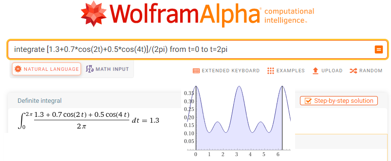

Fig. 11-10
Calculation of the sc0 centroid for F(0j1t)=[1.3+0.7cos(2t)+ 0.5cos(4t)]/(2pi)
The centroid sc0=(1.3,0) centroid=1.3 for the non-rotating trajectory of the function f(t)
is its constant component, i.e. the coefficient c0=a0=1.3 of the Fourier Series.
Chapter 11.5.3 Center of gravity sc2 for ω=2/sec
So sc2 trajectory F(-2j1t)=[1.3+0.7cos(2t)+0.5cos(4t)]*exp(-2j1t) for Fig. 11-9 ω=-2/sec
Click https://www.wolframalpha.com 
Enter or paste integrate [1.3+0.7*cos(2t)+0.5*cos(4t)]*exp (-2i1t)]/(2pi) from t = 0 to t = 2pi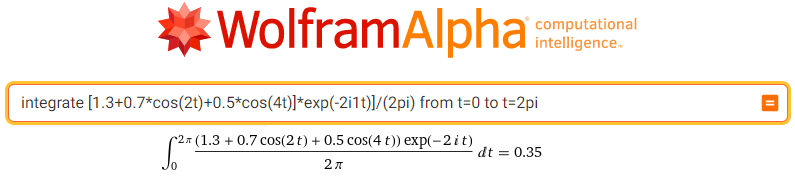 

Fig. 11-11
Calculation  sc2 of the centroid for F (2j1t)=[1.3+0.7cos (2t) + 0.5 cos (4t)]*exp (-2j1t)/(2pi)
The centroid sc2=0.35=(0.35.0) , i.e. the 2nd harmonic amplitude is c2=2(0.35.0]=(0.7,0). i.e. a2=0.7 b2=0
The second harmonic is h2(t)=0.7cos(2t) acc. Fig. 11-1h.
Chapter 11.5.4 Centroid sc3 for ω=3/sec
So sc3 trajectory F(-3j1t)=[1.3+0.7cos(2t)+0.5cos(4t)]*exp(-3j1t) for Fig. 11-9 ω=-3/sec
Click https://www.wolframalpha.com 
Enter or paste integrate [1.3+0.7cos(2t)+0.5cos(4t)]*exp(-3j1t)]*exp (-3i1t)]/(2pi) from t=0 to t=2pi 

Fig. 11-12
Calculation of the sc3 centroid of the trajectory [1.3+0.7cos (2t)+0.5cos(4t)]*exp (-3j1t)/(2pi)
The centroid sc3=0=(0,0) , i.e. 3rd harmonic amplitude c3=2*0=0.There is no third harmonic. There is also no 5,6,7 … harmonics.
You can see this in the f(t) function itself, of course, but you can check it with WolframAlfa.
Chapter 11.5.5 Centroid sc4 for ω=4/sec
So sc4 trajectory F(-4j1t)=[1.3+0.7cos(2t)+0.5cos(4t)]*exp(-4j1t) for Fig. 11-9 ω=-4/sec
Click https://www.wolframalpha.com 
Enter or paste integrate [1.3+0.7*cos(2t)+0.5*cos(4t)]*exp(-4i1t)]/(2pi) from t = 0 to t = 2pi 
Fig. 11-13
Calculation of the sc4 centroid for F(4j1t)=[1.3+0.7cos (2t)+0.5 cos (4t)]*exp (-4j1t)/(2pi)
Centroid sc4=0.25=(0.25.0) , i.e. the 4th harmonic amplitude is c4=2(0.25.0]=(0.5,0). i.e. a4=0.5 b4=0
The fourth harmonic is h4(t)=0.5cos(4t) acc. Fig. 11-1h.

Chapter 11.6 Centroids of trajectory F(nj1t)=0.5cos(4t-30°)*exp(-4j1t)
for n = 0.2,3.4 and ω0=1/sec that is with completely complex type numbers
Until now, the centroidsy scn of the harmonics were real numbers, eg Fig. 11-9 ω=-2/sec–->sc2=(0.35.0)= 0.35. They are also complex numbers, but with zero imaginary components. What if the cosine function has a phase shift?
So let’s throw into the centrifuge e.g. f(t)=0.5cos(4t-30 °).
Let us turn the rotation to n=0, n=1 and n = 4.
There will be 3 trajectories:
n=0–>ω=0–> centrifuge is standing–> F(-0j1t)=0.5cos (4t-30 °)
n=1–>ω=-1/sec–>centrifuge is rotating–>F(-1j1t)=0.5cos(4t-30 °)*exp (-1j1t)
n=4–>ω=-4/sec –>centrifuge is rotating–>F(-4j1t) = 0.5cos (4t-30 °)*exp (-4j1t)

Fig. 11-14
F(nj1t)=0.5cos(4t-30°)*exp(-jnt) for n=0,1 i 4
The animation lasts T=2π≈6.28sec.
ω=0
F(0j1t)=0.5cos(4t-30°)
The difference between the animation Fig. 11-5 ω=0 is minimal, but try to notice it.
ω=-1/sec.
F(4j1t)=0.5cos(4t-30°)*exp(-j1t)
The trajectory is rotated by (I suspect?)-30° relative to Fig. 11-5 ω=-1/sec. The centroid sc0=(0,0). This means that there is no harmonic of the function f(t)=0.5cos(4t) for ω=1/sec. Also for any other, except for ω=4/sec.
ω=-4/sec.
F(4j1t)=0.5cos(4t-30°)*exp(-4j1t)
The centroid sc4 is a full-fledged complex number sc4=(a,b) where:
a=0.25cos(-30°)≈+0.217
b=0.25sin(-30°)≈-0.125
sc4=(a,b)≈(+0.217,-0.125)=+0.217-j0.125
So the complex fourth harmonic h4(t)≈2*sc≈2*(+0.217-j0.125)*exp(j4t). It corresponds to the function f(t)=0.434cos(4t)+0.25sin(4t)=0.5cos (4t-30°) according to the formulas Fig. 11-1h and Fig. 11-1i What does WolframAlfa say?
Click https://www.wolframalpha.com.
Enter or pastej integrate [0.5cos(4t-pi/6)]/(2pi)*exp(-4i1t) from t=0 to t=2pi
Note  -30° =-π/6

Fig. 11-15
sc4=0.216506-j0.125
Such centroid sc4 of the trajectory F(4j1t)=0.5cos(4t-30°)*exp (-j4t) was calculated by WolframAlfa. A result similar to ours, only more accurate. Note that sc4 is a full complex number. This is the case when the cosine/sinus type function has a non-zero
phase shift ϕ. Here ϕ=30°=-π/6.
Fun fact
Compare the animations Fig. 11-13 ω=-1/sec and ω=-4/sec.
ω=-1/sec
Four Leaf Clover
ω=-4/sec
It is also some kind of a leafy clover except that each leaf is a circle and is drawn “on top of each other”. 

Chapter 11.7 Centroids of trajectories
F(-njω0t)=[0.5+1.08cos (1t-33.7 °)+0.72cos(3t+33.7°)+0.45cos(5t-26.6 °)]*exp(-njω0t)
for n = 0,1,2…8 and ω0=1/sec
Chapter 11.7.1 Introduction
The function f(t) with the period T=2πsec looks like this and you don’t see its 3 cosines with phases ϕ. Otherwise WolframAlfa theoretical doesn’t need to know the formula  f(t). For him, the f(t) diagram alone is enough.|

Fig. 11-16
f(t)=0.5+1.08*cos(1t-33.7°)+0.72*cos(3t+33.7°)+0.45*cos(5t-26.6°)
In Chapter 6 we examined 9 trajectories F(-njω0t) of this function f(t) for n=0,1,2,… 8 and ω0=1/sec. It is interesting because due to the phase shifts ϕ, the scn centroids are completely complex numbers. The function f(t) is equivalent to the following, in which each harmonic has been decomposed into a cosine and a sinusoidal component–> f(t)=0.5+0.9cos(1t)+0.6sin(1t)+0.6cos(3t)-0.4sin(3t)+0.4cos(5t)+0.2sin(5t).
e.g. 0.9*cos(1t)+0.6*sin(1t)=1.08*cos(1t-33.7°)
This is the same function, but complex Fourier coefficients, or complex Fourier amplitudes, are easily determined here. From them, harmonics are read as h1(t), h3(t) and h5(t) waveforms with sine/cosine components.
c1=0.9-j0.6—>h1(t)=0.9*cos(1t)+0.6*sin(1t)
c3=0.6+j0.4–>h3(t)=0.6*cos(3t)-0.4*sin(3t)
c5=0.4-j0.2—>h5(t)=0.4*cos(5t)+0.2*sin(5t)
Note:
Both forms of the function f(t) are equivalent, but for the calculations we will take the version with “cosines and sines”. We will put the functions f(t) into the centrifuge with different speeds nω0=-n/sec for n=0,1,2,3 and 5. We will check if the calculated  scn centroids are the same as in Chapter 6.
Chapter 11.7.2 Centroids scn of trajectory F(-njω0t)=f (t)exp(-njω0t) for n = 0, 1,2, 3, 5 and ω0=1 sec
Let’s put the function from Fig. 11-15 into the centrifuge. I would like to remind you that it can also be presented in the sine/cosine version, i.e: f(t)=0.5+0.9cos(1t)+0.6sin(1t)+0.6cos(3t)-0.4sin(3t)+0.4cos(5t)+0.2sin(5t).
Let’s turn on the rotation for n=0, 1, 2, 3 and 5. So for the speeds ω=0 (the centrifuge is standing!), ω=-1/sec, ω=-2/sec, ω=-3/sec and ω=-5/sec. The formation of 5 trajectories:
ω=0–>centrifuge is standing–>F(-0j1t)=f(t)
ω=-1/sec–>centrifuge is rotating—>F(-1j1t)=f(t)exp(-1j1t) 
ω=-2/sec–>centrifuge is rotating—>F(-2j1t)=f(t)exp(-2j1t)
ω=-3/sec–>centrifuge is rotating—>F(-3j1t)=f(t)exp(-3j1t)
ω=-5/sec–>centrifuge is rotating—>F(-5j1t)=f(t)exp(-5j1t)

Fig. 11-17
5 trajectories F(-nj1t)=f t)exp (nj1t) for n = 0,1,2,3 and 5 ω=0 and their  scn centroids.
ω=0
The centrifuge is standing and sc0=(+ 0.5.0)
ω=-1/sec 
Rotating ω=-1/sec –>sc1=(+0.45,-0.3)
ω=-2/sec 
Rotating  ω=-2/sec –>sc2=(0,0)
ω=-3/sec 
Rotating  ω=-3/sec –>sc3=(+0.3,+0.2)
ω=-5/sec
Rotating  ω=-5/sec–>sc5=(+0.2,-0.1)
Let me remind you that the vector scn is almost the nth harmonic of the periodic function f(t). More specifically, the doubled vector i.e. 2scn is the complex amplitude of the nth harmonic. In the period T=2π sec, each trajectory is drawn by a changing vector and scn is the average of these changing vectors and therefore their sum is divided by 2π.
Chapter 11.7.3 Centroid sc0, i.e. for ω=0
Trajectory F(0j1t)=f(t) from Fig. 11-16 ω=0.
The centrifuge is standing. The trajectory is the horizontally swinging line in Fig. 11-17 ω=0 acc. to the function F(0j1t)=f(t). Its centroidy is sc0=(+0.5,0)=+0.5.
Let’s put f(t) into the formula Fig. 11-1c.
Click https://www.wolframalpha.com and do what the picture tells you to do. Enter or paste the WolframAlfa instruction.
integrate [0.5+0.9*cos(1t)+0.6*sin(1t)+0.6*cos(3t)-0.4*sin(3t)+0.4*cos(5t)+0.2*sin(5t)]/(2pi) dt from t=0 to t=2pi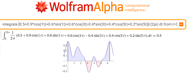

Fig. 11-18
Calculation of the centroid sc0 for F(0j1t)=f(t)/(2pi)
You see sc0 as a surface of the f(t) ((divided  by 2π). Note that they are plus and minus sufaces.
The centroid sc0=(0.5,0)=a0=0.5 for the non-rotating trajectory of the function f(t) is its constant component, i.e. the coefficient c0=a0 of the Fourier Series.
Chapter 11.7.4 Centroid sc1 for ω=1/sec.
Trajectory F(-1j1t)=f(t)exp(-1j1t) from Fig. 11-17 ω=-1/sec
Click https://www.wolframalpha.com. Type or paste into the box
integrate [0.5+0.9*cos(1t)+0.6*sin(1t)+0.6*cos(3t)-0.4*sin(3t)+0.4*cos(5t)+0.2*sin(5t)]*exp(-1i1t)]/(2pi) dt from t=0 to t=2pi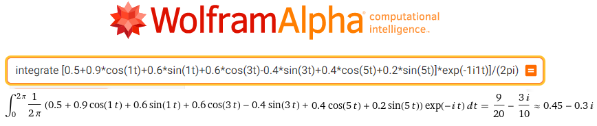

Fig. 11-19
Trajectory  F(-1j1t)=f(t)*exp(-1j1t)
Note:
In the window, you only see the part of the expression you pasted.
The calculated centroid is sc1=0.45-j0.3
The complex amplitude of the first harmonic is 2sc1=0.9-j0.6
So the first harmonic according to Fig. 11-1h and Fig. 11-1i is:
h1(t)=0.9cos(1t)+0.6sin(1t)=1.08*cos(1t-33.7°).
Success! WolframAlfa perfectly filtered the first harmonic from the periodic function f(t). We expect the same in the following chapters.
Chapter 11.7.5 Centroid sc2 for ω=2/sec.
Trajectory F(-2j1t)=f t)exp(-2j1t) from Fig.11-17 ω=-2/sec
Click https://www.wolframalpha.com.
Type or paste into the box
integrate (0.5+0.9*cos(1t)+0.6*sin(1t)+0.6*cos(3t)-0.4*sin(3t)+0.4*cos(5t)+0.2*sin(5t))*exp(-2i1t)/(2pi) dt from t=0 to t=2pi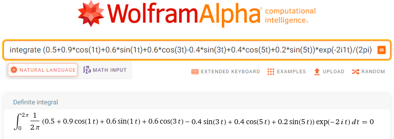

Fig. 11-20
Trajectory F(-2j1t)=f(t)*exp(-2j1t)
sc2=0
That is, there is no harmonic with pulsation ω=2/sec
Chapter 11.7.6 Centroid sc3 for ω=3/sec.
Trajectory F(-3j1t)=f t)exp(-3j1t) from Fig. 11-17 ω=-3/sec
Click https://www.wolframalpha.com.
Type or paste into the box
integrate (0.5+0.9*cos(1t)+0.6*sin(1t)+0.6*cos(3t)-0.4*sin(3t)+0.4*cos(5t)+0.2*sin(5t))*exp(-3i1t)/(2pi) dt from t=0 to t=2pi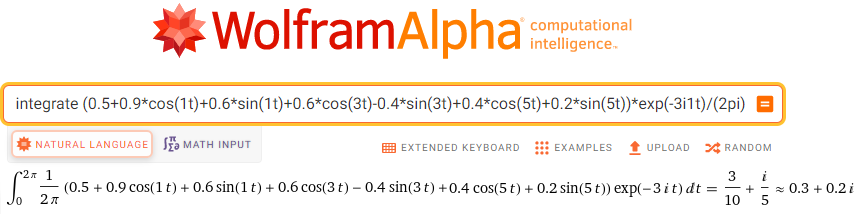

Fig. 11-21
Trajectory F(-3j1t)=f(t)*exp(-3j1t)
The calculated centroid is sc3=0.3+j0.2
The complex amplitude of the third harmonic is 2sc1=0.6-j0.4
So the third harmonic according to Fig. 11-1h and Fig. 11-1i is:
h3(t)=0.6cos(3t)-0.4sin(3t)≈0.72*cos(3t+33.7°)..
Chapter 11.7.7 Centroid sc5 for ω=5/sec.
Trajectory F(-5j1t)=f t)exp(-5j1t) from Fig. 11-17 ω=-5/sec
Click https://www.wolframalpha.com.
Type or paste into the box
integrate (0.5+0.9*cos(1t)+0.6*sin(1t)+0.6*cos(3t)-0.4*sin(3t)+0.4*cos(5t)+0.2*sin(5t))*exp(-5i1t)/(2pi) dt from t=0 to t=2pi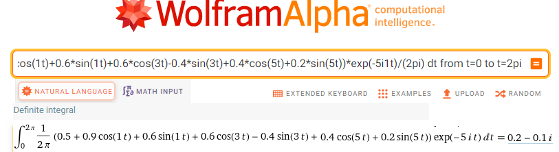

Fig. 11-22
Trajectory F(-5j1t)=f(t)*exp(-5j1t)
The calculated centroid is sc5=0.2-j0.1
The complex amplitude of the third harmonic is 2sc1=0.4-j0.2
So the fifth harmonic according to Fig. 11-1h and Fig. 11-1i is:
h5(t)=0.4cos(5t)+0.2sin(5t)≈0.45*cos(5t-26.6°)
Chapter 11.7.8 Centroids scn of the trajectories F (-njω0t)=f (t)exp(-njω0t) for n= 4,6,7,8 and ω0=1/sec
There are still centroids sc4, sc6, sc7 and sc8 i.e. for n=4,6,7 and 8. They are zero, i.e. there are no harmonics for these pulsations. I suggest you make the calculations yourself with the WolframAlfa program. 

Chapter 11.8 Centroids scn of the even square wave trajectory for n=0,1,2,… 8 and ω0=1/sec
Chapter 11.8.1 Introduction
We will repeat chaper 8, but this time we will calculate the centroids of the trajectory scn using the WolframAlfa program. Previously, we took them on faith.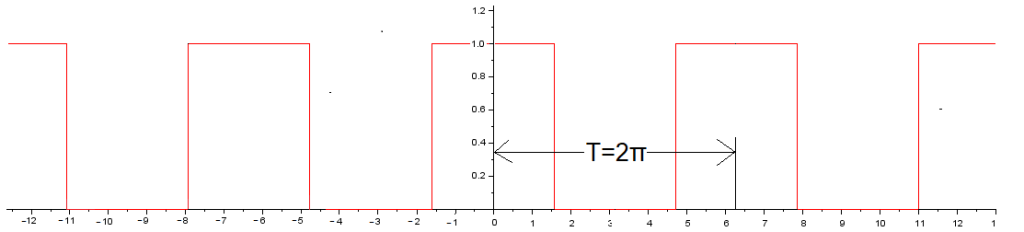

Fig. 11-23
Even square wave f(t) A=1, ω=1/sec, ϕ=0 and ω=50%.
We will calculate the successive harmonics with the WolframAlfa program using the formulas Fig. 11-1. But first we will check how WolframAlfa deals with square waves.
Chapter 11.8.2 Square wave f t) and WolframAlfa
We know what an instruction of a function looks like, e.g. sin(t) in WolframAlfa.
The function sin(t) is just sin(t) and the natural logarym ln(t) is ln(t). A square wave, on the other hand, is squarewave[t].
Let’s plot this function with the plot instruction.
Click https://www.wolframalpha.com.
Type or paste into the box
plot squarewave[t] from t=-2 to 2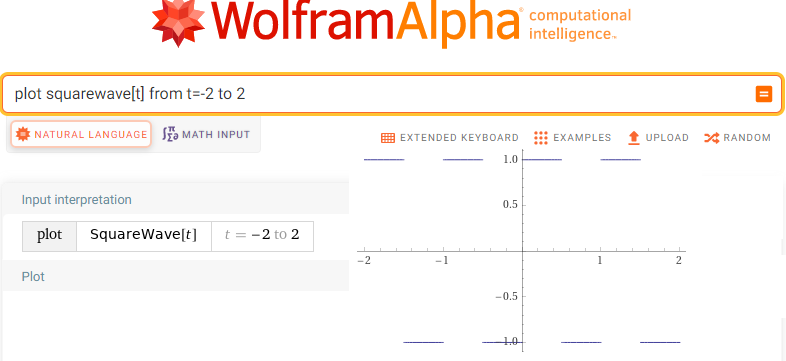

Fig.11-24
Squarewave[t] from t=-2 to 2
It is an odd, periodic function T = 1sec, A = 2 without a constant component. How to modify it to get the even as in Fig.11-23?
One should
1. Multiply by 0.5 to reduce the amplitude from A=2 to A=1
2. “Stretch” from T=1sec to T=2πsec
3. Move to the left π/2sec to change the odd function to even.
4. Move up 0.5
Let’s test it
Click https://www.wolframalpha.com.
Type or paste into the box
plot 0.5*squarewave[(t+0.5pi)/(2pi)]+0.5 from t=-2π to 2π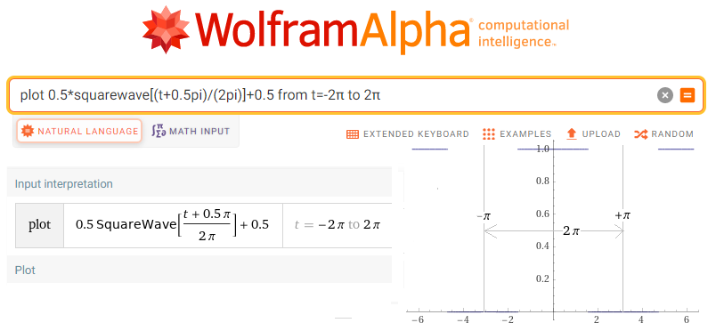

Fig.11-25
The square wave from Fig. 11-23 generated by the WolframAlfa program.
The period T=2π is shown, more precisely from -π to + π.
In the following chapters we will designate its trajectories, centroids scn and harmonics hn(t).
Chapter 11.8.3 Centroid sc0, that is for ω = 0, that is the constant component a0.
We will use the formula Fig. 11-1c
Click https://www.wolframalpha.com.
Type or paste into the box
(1/(2pi))*integrate [[0.5+ 0.5 * SquareWave [(t + pi/2)/(2pi)]] from t=-pi to t=+pi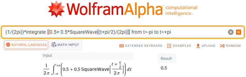

Fig.11-26
Calculation the constant component sc0=c0=a0=+0.5
As expected, a0=0.5 as the mean value of the square wave over the period -π to + π.
It was not even necessary to integrate, because a0 as the mean can be seen in Fig. 11-25.
Chapter 11.8.4 Centroid sc1, that is for ω=-1/sec.
So sc1 of the trajectory F (-1j1t)=f (t)exp(-1j1t) where f(t) is a square wave from Fig. 11-25.
We will repeat the animation from Fig. 8-3 chapter. 8.

Fig. 11-27
Trajectory F (1j1t) of an even square wave
a. Vector 1exp(1j1t) as radius R=1 rotating at speed ω=-1/sec
b. Vector F(1j1t) as a radius R=1 modulated by a square wave f (t) from Fig. 11-25.
c. Trajectory F(1j1t) of an even square wave drawn by the vector b.
The vector of the centroid of the trajectory sc1=(+1 /π, 0) more or less agrees with the intuition, But as the mean of the rotating vector b must lie somewhere between (0,0) and (1,0).
Now let’s count it exactly with the WolframAlfa program. We will use the formula Fig. 11-1c.
Click https://www.wolframalpha.com. Type or paste into the box
[(1/(2pi)]*integrate[[0.5+0.5*SquareWave[(t+pi/2)/(2pi)]]*exp(-1i1t) dt from t=0 to t=+2pi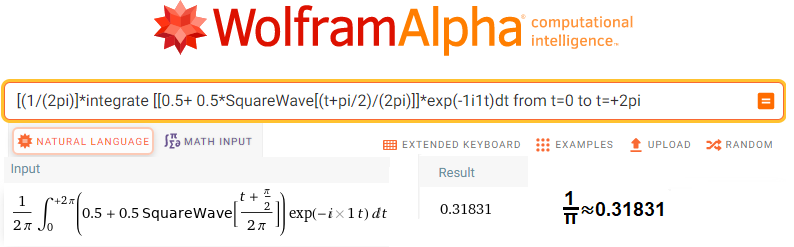

Fig. 1-28
Calculation of sc1=(1/ π, 0)
The program calculated the average of the vectors over time T=2πsec and it came out 0.31831.
First, it calculated a more precise value but rounded to 5 decimal places.
Second, it is exactly the number 1/π
Third, it is a vector in the form of a complex number sc1=(1/π, 0)
Chapter 11.8.5 Centroid sc2=0, that is for ω=-2/sec.
So sc2 of the trajectory F(-2j1t)=f(t)exp(-2j1t) where f(t) is a square wave from Fig. 11-23. We will repeat the animation from Fig. 8-5 chapter. 8.

Fig. 11-29
Trajectory F(2j1t) of an even square wave
a. Vector 1exp (j2j1t) as radius R=1 rotating at speed ω=-2/sec
b. Vector F(2j1t) as radius R=1 modulated by square wave f(t) from Fig. 11-25.
c. Trajectory F(2j1t) of an even square wave drawn by the vector b. The trajectory centroid sc2=(0,0) agrees as the mean.
Now let’s calculate it exactly with the WolframAlfa program.
Click https://www.wolframalpha.com. Type or paste into the box
[(1/(2pi)]*integrate [[0.5+ 0.5*SquareWave[(t+pi/2)/(2pi)]]*exp(-2i1t)dt from t=0 to t=+2pi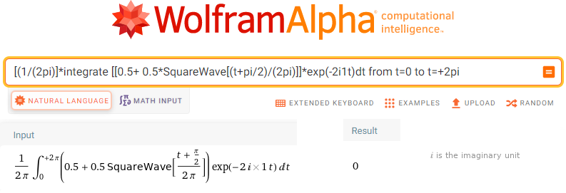

Fig. 11-30
Calculation sc2=0=(0,0)
That is, the second harmonic, more precisely for ω=2/sec, doesn’t exist
Chapter 11.8.6 Centroid sc3, that is for ω=-3/sec.
So sc3 trajectory F(-3j1t)=f (t)exp(-3j1t) where f (t) is a square wave from Fig. 11-25. We will repeat the animation from Fig. 8-6 chapter. 8.

Fig. 11-31
Trajectory F(3j1t) of an even square wave
a. Vector 1exp (j3j1t) as radius R=1 rotating at speed ω=-3/sec
b. Vector F(3j1t) as radius R=1 modulated by square wave f(t) from Fig. 11-25.
c. Trajectory F(3j1t) of an even square wave drawn by the vector b
Vector of the centroid of the trajectory sc3=(-1/3π, 0). The animation b is best suited for interpretation. Notice that the vector makes 2×3/4 turns. The left direction of the vector on the Re z axis is obvious when we consider 2 empty quarter turns. If they were not there (2×1 turn), then sc3=(0,0). And why is the length of the vector sc3 smaller than the length of sc1 in Figure 11-27c? Because there are more gaps in the period T=2πsec, which reduces the average. Ultimately, WolframAlfa will convince you.
We will use the formula Fig. 11-1c
Click https://www.wolframalpha.com.
Type or paste into the box
[(1/(2pi)]*integrate [[0.5+ 0.5*SquareWave[(t+pi/2)/(2pi)]]*exp(-3i1t)dt from t=0 to t=+2pi

Fig.1-32
Calculation sc3=(-1/3π,0)
Chapter 11.8.7 Centroid sc4=0, that is for ω=-4/sec.
So sc4 of the trajectory F(-4j1t)=f (t)exp (-4j1t) where f (t) is a square wave from Fig. 11-25. We will repeat the animation from Fig. 8-5 chapter. 8.

Fig. 11-33
Trajectory F(4j1t) of an even square wave
a. Vector 1exp(4j1t) as radius R=1 rotating at speed ω=-4/sec
b. Vector F(4j1t) as radius R=1 modulated by square wave f (t) from Fig. 11-25.
c. Trajectory F(4j1t) drawn by the vector from b.
The trajectory center of gravity vector sc4=(0,0) agrees as the mean.
Now let’s count it exactly with the WolframAlfa program. We will use the formula Fig. 11-1c
We will use the formula Fig. 11-1c
Click https://www.wolframalpha.com.
Type or paste into the box
[(1/(2pi)]*integrate [[0.5+ 0.5*SquareWave[(t+pi/2)/(2pi)]]*exp(-4i1t)dt from t=0 to t=+2pi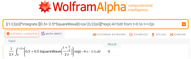

Fig. 11-34
Calculation sc4=0=(0,0)
That is, the fourth harmonic, more precisely for ω=4/sec, doesn’t exist
Chapter 11.8.8 Centroid sc5, sc6, sc7 and sc8, that is for ω = -5 / sec, -6 / sec, -7 / sec and- 8 / sec.
As homework. I will just suggest that it is enough to paste it into the WolframAlfa window [(1/(2pi)]*integrate [[0.5+ 0.5*SquareWave[(t+pi/2)/(2pi)]]*exp(-ni1t)dt from t=0 to t=+2pi
with an appropriately changed parameter n.