2. The complex function exp(jωt) as a model of the real function cos(ωt)

Rotating Fourier Series

Chapter 2. The complex function exp(jωt) as a model of the real function cos(ωt)

2.1 Introduction
The purpose of this article is to treat sine/cosine as rotating vectors. For example, a vector 1 rotating at a speed of ω0=1/sec, more precisely (1,0) corresponds to the real function 1*cos(ω0t)=1*cos(1t). Let me remind you that the angular velocity ω0=1 (more precisely ω0=1/sec) has a period T=2π sec≈6.28sec. This approach will greatly facilitate the intuitive understanding of the formulas related to the Fourier Series, Fourier Transform and Laplace Transform.
Note on ω0 pulsation.
And why not just ω? Because this is an article on Fourier Series and ω0 is the pulsation of the fundamental harmonic*, and ω=n*ω0 is about the nth harmonic of the periodic function f(t).
*Some call the ω0 pulsation the ω1–first harmonic pulsation.

Chapter 2.2 Euler’s equation
I assume you are familiar with complex numbers and the complex function exp(jω0t), which are used in many fields. For me an electrician, these are rotating vectors. They show better the phase shifts ϕ between current and voltage than on ordinary time charts. If you don’t feel confident, I recommend the “Complex Numbers” course on the home page.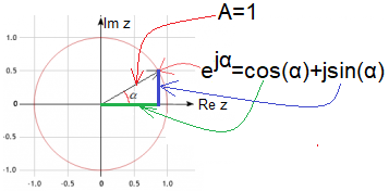

Fig. 2-1
Euler’s equation
Treat the angle α generally as a good x, i.e. as a real number related to the equation! And jα is an imaginary number on the Im z axis. Only this equation results in its interpretation with a circle and a right triangle. Here it is clear that the real number α is the angle in radians. For any real number α, the complex value z=exp(jα) will be somewhere on a circle with radius A=1. At first glance, it seems as obvious as the definitions of sine and cosine. But what does the complex exponent function exp(jα) have to do with trigonometry? Mr. Euler in his time could only use complex addition, subtraction, multiplication and division. What about the complex function exp(jω0t)? How to calculate it using only the above four operations? However, Euler already knew that the real function exp(x) is a sum of infinitely many decreasing polynomials, just like the number 1 is an infinite sum of the series 1/2+1/4+1/8+1/16+… Similarly treated the complex exponential function exp(jx). i.e. calculated its value as a sum of polynomials using only four complex number operations. And he must have been surprised when the point z=exp(jx) started rotating in a circle with radius A=1. Only then did he associate x with the angle α. And he expected the function to go somewhere to infinity. Just like the real exponential function exp(x) for x>0! Substitute into Euler’s formula α=0, 0.25π, 0.5π, 0.75π …2π in sequence. You will see the point z=exp(jα) rotating in a circle.

Chapter 2.3 Video support
The main advantage of the article is the animation. It is much more imaginative than a simple chart.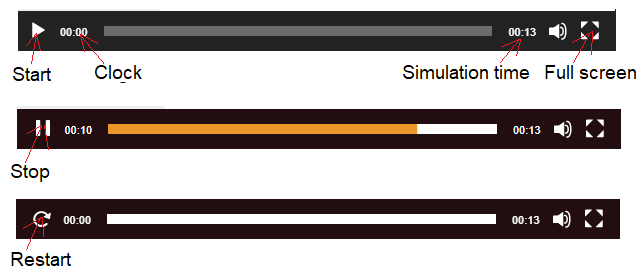

Fig. 2-2
Description of buttons and video indicators
– Start clicking starts the animation and turns into a Stop button
– Clock the current time of the experiment, also as a yellow bar
– Simulation time otherwise – the duration of the experiment, here 13 sec.
– Full screen click to enlarge the screen, click again to reduce etc…
-Stop Clicking stops the simulation and changes to a Restart button
-Restart as the name suggests.

Chapter 2.4 Study of various harmonic motions f(t) as their two-dimensional versions F(jω0t)
This chapter is just an excuse to get acquainted with the complex function Start*exp(jω0t). I emphasize that the parameters Start and jω0t are complex numbers! Now that we know how to handle video, we will examine the harmonic motions for different initial states of the rotating Start vector and the ω0 pulsation. You’ll see that the time function x(t) is the projection of the rotating vector Start*exp(jω0t) onto the real axis Re z. So x(t)=Re z {Start*exp(jω0t)}.
We will examine 5 harmonic movements.
1. 1cos(1t) as Start*exp(jω0t) for Start=1 and ω0=1/sec
2. 1sin(1t) as Start*exp(jω0t) for Start=1*exp(-jπ/2)=1*exp(-j90°)=-1j and ω0=1/sec
3. 1cos(1t-π/4) as Start*exp(jω0t) for Start=1*exp(-jπ/4)=1*exp(-j45°)≈0.707-j0.707 and ω0=1/sec
4. 1cos(2t) as Start*exp(jω0t) for Start=1 and ω0=2/sec
5. 0.5cos(1t) as Start*exp(jω0t) for Start=0.5 and ω0=1/sec
Chapter 2.4.1 f(t)=1*cos(1t) as F(jω0t)=1*exp(j1t) that is Start*exp(jω0t) for Start=1 and ω0=1/sec
The most important conclusion:
The rotating vector F(jω0t)=1*exp(j1t) is a two-dimensional version of f(t)= x(t)=1*cos(1t). Here ω0=1/sec.
Later it will turn out that almost every arbitrary periodic function f(t) with period T corresponding to the pulsation ω=2π/T has its two-dimensional version as the sum F(jt)=c1*exp(j1ω0t)+c2*exp(j2ω0t)+c3 *exp(j3ω0t)…
c1, c2, c3… are complex numbers or vectors an+jbn as initial states of rotating vectors cn*exp(jnω0t).
In the two-dimensional version F(jω0t) of the function f(t), some features are more visible and intuitive than in the one-dimensional one–>f(t).

Fig. 2-3
Fig. 2-3a
x(t)=1cos(1t)
This is one-dimensional motion along the real axis Re z in the complex plane Re z, Im z. Click the “Start” button to see the 2 periods T of harmonic motion. We know the amplitude A=1 and the time of the 2 periods, i.e. 2T≈12 sec≈12.56 sec≈4πsec shown on the video stopwatch, i.e. T=2πsec–>ω0=2/T=1/sec. The absolute values of the speed are the highest in the middle, and the smallest, i.e. zero, at the ends “at the turns“.
Fig. 2-3b
The complex function 1exp(jω0t) as a rotating vector of length 1 and initial state (1,0)
Note:
Start=z=(1,0)=1+0j. It is the complex function that has the value Start*exp(j1t)=(1+0j)*exp(j1t)=1*exp(j1t) and is a rotating vector of length 1 and initial state (1,0). It is clearly visible that the animation in Fig.2-3a is a projection of the animation in Fig.2-3b onto the real axis Re z.
Or otherwise
“The real part of the complex function 1exp(j1t) is the function 1cos(1t).
Or otherwise
Re 1exp(j1t)=1cos(1t)
The projection of the rotating vector onto the real axis Re z moves as in Fig. 2-3a.
Some people almost equate exp(jω0t) with cos(ω0t). It’s not exact, but it’s accurate and visual.
The initial state of the circulating vector Start=(1+0j)=+1 you can see in Fig. 2-3b before the animation.
Remember, I won’t repeat it a second time!
Each Start vector is the initial state and “stands still”. Here Start=z=1+0j, but it can be e.g. Start=z=2-3j.
After multiplying Start by exp(jω0t), the vector Start*exp(jω0t) will start to rotate at a speed of ω0. You will also find out about it in the next animations.
Fig. 2-3c
Time chart x(t)=1cos(1t) (ω0=1/sec)
– the horizontal axis (“x”) is time t in seconds.
Keypoints 0 sec, 0.5πsec≈1.57sec, 0.75πsec≈2.36sec, πsec≈3.14sec, 2πsec≈6.28sec
– the vertical axis (“y”) is x(t) in units
Try to stop the simulation “more or less” at these times and compare Fig. 2-3a, Fig. 2-3b and Fig. 2-3c.
Chapter 2.4.2 f(t)=1*sin(1t) as F(jt)=Start*exp(jω0t) for Start=-1j and ω0=1/sec

Fig. 2-4
Fig. 2-4a
x(t)=x(t)=1sin(1t)
This is the projection of the circulating vector from Fig. 2-4b onto the real axis Re z.
Fig. 2-4b
Complex function -1j*exp(j1t) for ω0=1/sec, otherwise exp(j1t-π/2)*exp(j1t) because -1j=exp(j1t-π/2)
Note:
Because the point Start=0-1j=-1j
This complex function has the value Start*exp(j1t)=-1j*exp(j1t).
You can see the initial state of the rotating vector Start=-1j in Fig. 2-4b before the simulation.
Compare with Fig. 2-3b. You can clearly see the truth known for centuries that sin(ω0t) is delayed by π/2 = 90º with respect to cos(ω0t).
Fig. 2-4c
Time chart x(t)=1sin(1t)
Chapter 2.4.3 f(t)=1*cos(1t-π/4) as F(jt)=Start*exp(jω0t) for Start=1*exp(-jπ/4)=0.707-j0.707 and ω0=1/sec

Fig. 2-5
Fig. 2-5a
x(t)=1cos(1t-π/4) or x(t)=Acos(ω0t-ϕ) for A=1 ω0=1/sec and ϕ=-π/4 = -45º
This is the projection of the circulating vector from Fig. 2-4b onto the real axis Re z.
Fig. 2-5b
The complex function 1*exp(j1t-π/4) as 1*cos(1t-π/4).
Note that the lag ϕ=-π/4 (ϕ=-45º) is beautiful here. Check with Pythagoras that the amplitude A=1
and that ϕ=-π/4=-45º.
We can write the circulating vector in different ways.
Start*exp(j1t)=exp(-jπ/4)*exp(j1t)=(1/√2-j1/√2)*exp(j1t)≈(0.707-j0.707)*exp(j1t).
You can see the initial state of the circulating vector Start=exp(-jπ/4) in Fig. 2-5b.
Fig. 2-5c
Time chart x(t)=1cos(1t-π/4)
Section 2.4.4 f(t)=1*cos(2t) as F(jt)=Start*exp(jω0t) for Start=1 and ω0=2/sec
We increased the speed to ω0=2/sec relative to Fig. 2-3.

Fig. 2-6
Rys. 2-6a
Time chart 2 times faster than in Fig. 2-3. Besides, the initial state Start is the same, i.e. Start=(1+0j)=+1
Compare with the corresponding animations in Fig. 2-3.
x(t)=1cos(2t).
Fig. 2-6b
Complex function 1exp(j2t) as 1cos(2t)
Fig. 2-6c
Time chart x(t)=1cos(2t)
Chapter 2.4.5 f(t)=0.5cos(1t) as F(jω0t)=Start*exp(jω0t) for Start=0.5 and ω0=1/sec

Fig. 2-7
Fig. 2-7a
Time amplitude 2 times lower than in Fig. 2-3. The initial state Start is the same, i.e. Start=(0.5+0j)=+0.5.
Compare with the corresponding animations in Fig 2-3.
x(t)=1cos(2t).
Fig. 2-7b
Complex function 0.5*exp(j1t) as 0.5*cos(1t)
Note:
Fig. 2-7c
Time chart x(t)=0.5cos(1t)

Chapter 2.5 Functions Start*exp(jω0t)
Compare again the previously discussed complex functions for different parameters Start and ω0.
1- Start=1 and ω0=1/sec
2- Start=1*exp(-jπ/2)=-j1 and ω0=1/sec
3- Start=1*exp(-jπ/4) and ω0=1/sec
4- Start=1 and ω0=2/sec
5- Start=0.5 and ω0=1/sec

Fig. 2-8
5 versions Start*exp(jω0t)
These functions are shown in Fig.2-4b…Fig.2-7b as rotating vectors. Their ends indicate points z whose coordinates are just complex functions Start*exp(j ω0t). The beetroot vector is the initial state of each function. This is the Start parameter that comes before exp(jω0t). Analyze each of the 5 waveforms carefully, taking into account the Start and ω parameters.
Compare, for example, Fig. 2-8b and Fig. 2-8a. Here, it is clearer than in the time plots that sin(1t)–>-j1exp(j1t) is lagged by 90° with respect to cos(1t)–>1exp(j1t).

Chapter 2.6 The complex function F(jt)=(a-jb)*exp(jω0t) as a two-dimensional version of f(t)=a*cos(ω0t)+b*sin(ω0t)
Chapter 2.6.1 General description
Dessert at the end. So how to build the trajectory F(jω0t) for any sine function f(t)=a*cos(ω0t)+b*sin(ω0t)=c*cos(ω0t-ϕ)
From Chapter 2.4.1 we know that the complex function 1*exp(jω0t) corresponds to the time chart 1*cos(ω0t).
Similarly, according to Chapter 2.4.2 of the complex function -1j*exp(jω0t) corresponds to 1*sin(ω0t).
We’ll write it like this:
1*exp(jω0t)<==>1*cos(ω0t)
–1j*exp(jω0t)<==>1*sin(ω0t)
This is the case with amplitudes a=1 for cosine and b=1 for sine.
This works for any amplitudes a and b:
a*exp(jω0t)<==>a*cos(ω0t)
-jb*exp(jω0t)<==>b*sin(ω0t)
Instead of writing that the function corresponds to something there, you can more precisely, as below.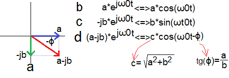

Fig. 2-9
Re (a-jb)*exp(jω0t)=a*cos(ω0t)+b*sin(ω0t)
Vector (a-jb) rotates with speed ω.
The projection of the rotating vector (a-jb)*exp(jω0t) on the real axis is:
real part (a-jb)*exp(jω0t)
that is, Re (a-jb)*exp(jω0t)=a*cos(ω0t)+b*sin(ω0t).
This is a generalization of the simplest case in Fig.2-3 where a=1 and b=0.
Fig. 2-9a
The complex function (a-jb)*exp(jω0t) as a vector rotating at ω0
It has 2 components:
-real (cosine) a*exp(jω0t)
-imaginary (sine) -jb*exp(jω0t)
What you see in Fig. 2-9a is the initial state of the rotating vector, i.e. for t=0.
I emphasize that “lonely” a and b are real numbers!
Fig. 2-9b
The projection of a rotating vector a*exp(jω0t) onto the real axis is a*cos(ω0t)
Fig. 2-9c
The projection of the rotating -jb*exp(jω0t) vector onto the imaginary axis is b*sin(ω0t)
Fig. 2-9d
The projection of the sum of the rotating vectors, the red vector, onto the real axis is a*cos(ω0t)+b*sin(ω0t)=c*cos(ω0t-ϕ)
It’s not very obvious, but that’s trigonometry! Instead of a proof*, let’s substitute a concrete one
values e.g. a=0.75 and b=1.25 and check the animation.
* This can be done by a high school student of the mathematics class.
Chapter 2.6.2 Concrete example F(jω0t)=(0.75-j1.25)*exp(jω0t) as a two-dimensional version of f(t)=0.75*cos(ω0t)+1.25*sin(ω0t)

Fig. 2-10
Rotating vector (0.75-j1.25)*exp(1jt) as f(t)=0.75*cos(1t)+1.25*sin(1t)=1.458*cos(1t-59.04°)
Fig. 2-10a
Rotating vector 0.75*exp(1jt) and its projection on the Re z axis as a function of time 0.75*cos(1t)
Fig. 2-10b
Rotating vector -j1.25*exp(1jt) and its projection on the Re z axis as a function of time 1.25*sin(1t)
Fig. 2-10c
Sum of 2 left vectors as rotating vector (0.75-j1.25)*exp(1jt)
Its projection on the Rez axis is a function of time f(t)=0.75*cos(1t)+1.25*sin(1t)=1.458*cos(1t-59.04°) and its time chart is shown in the animation below.

Fig. 2-11
1.458*cos(1t-59.04°)=0.75*cos(1t)+1.25*sin(1t)
An angular offset of 59.04° ≈1.03 radian is shown in the time chart.