7. How to calculate centroids of scn trajectories and harmonics detector.

Rotating Fourier Series

Chapter 7. How to calculate centroids of scn trajectories and harmonics detector.

Chapter 7.1 Introduction
In chapter 4 (4.5, 4.6), we extracted from the rotating trajectory F(njω0t) its “centre of gravity” or “centroid” scn as a complex number. And this is almost the nth harmonic with the pulsation ω=n*ω0 of the function f(t). At that time, we did not know the formula for scn and we accepted the result without proof. Now we will get to know it in Fig. 7-2b,c as well as the relationship of the centroid scn of the nth trajectory with the nth harmonic f(t) in Fig. 7-2i,j.

Chapter 7.2 The centroids of trajectories and harmonics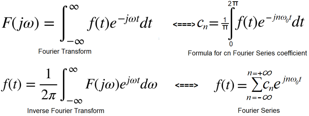

Fig. 7-1
Strange Formulas
Don’t go into details for now. Let me just say that formulas are among the most important in mathematics, just like mc_square in physics. They are not intuitive, because what is not here? Complex functions, integrals, infinities, ω pulsations. The equations correspond to some trajectories in the complex plane. And the so-called the “center of gravity” or “centroids” of the trajectories will make it much easier to understand these strange and difficult formulas.

Chapter 7.3 Centroid scn of the trajectory F(njωot) of the function f(t) rotating at speed -nω0.
The centroid scn (center of gravity) for the nth F(njωot) trajectory is a complex number from which we can easily read the nth harmonic of the f(t) function with ω=n*ω0 pulsation. As if we threw a periodic function f(t) into a centrifuge rotating at a speed of ω=n*ω0. And what comes out of it? Of course it’s a harmonic with pulsation ω=n*ω0! So far, we have determined the centroid of the scn intuitively. In simple cases where scn=(0,0) this was as expected. Such as, for example, the centroid of a circle. Now it’s time for the exact formula for the scn. There will be no strict proof. However, I will try to make it as obvious as riding a bike. Although is cycling obvious? The first cyclists in the 19th century were treated like circus performers. How does it move and not fall over?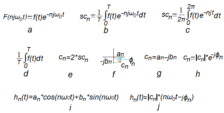

Fig. 7-2
Relation of the centroid scn of the trajectory F(njω0t) to the complex Fourier coefficients c0, cn=an-jbn* and the harmonics hn(t) of the function f(t) of period T.
* It seems that the formula 7-2g as cn=an+jbn would be more natural.
But then the formula 7-2i would appear in Fourier Series as hn(t)=an*cos(nω0t)-bn*sin(nω0t).
Fig. 7-2a
Trajectory F(njω0t)
The point moves on the real axis Re Z according to the periodic function f(t). When the centrifuge (Z plane) with the function f(t) rotates with the speed -nω0 (sign -, because “clockwise”), the trajectory is drawn according to complex function F(njω0t). For n=0, the centrifuge is stationary. The concept of a trajectory is already familiar to you after Chap. 4.5 and 6. If something is wrong, I recommend at least p. 4.3 from chapter 4.
Fig. 7-2b
General formula for the centrroid scn of the trajectory F(njω0t).
The integrand function is the trajectory F(njω0t). The integral (divided by 2T) can be treated as the point scn, the average distance of the trajectory F(njω0t) from (0,0) in the period T sec*. Then for n=1 the trajectory F(njω0t) will make 1 rotation in the period T=2π/1ω0, for n=2–> 2 rotations etc… But always in the same period T, only with a higher speed ω!
*If such a definition of the centroid of the trajectory F(njω0t) is not convincing, it may help chapter. 7.7
Fig. 7-2c
For functions that are “similar in time”, eg square waves with a duty cycle of 50% and amplitudes A=1 but with different pulsations, the centroids scn do not depend on the pulsations ω. They are the same for ω=1/sec and ω=1000/sec! Therefore, in the formula Fig. 7-2b we can assume ω=1/sec and the simplified formula Fig. 7-2c will be obtained. More on this topic in chapter 7.6
Fig. 7-2d
The formula for the c0 coefficient of the Fourier Series for n=0.
This is a constant component of f(t) and is therefore always a real number sc0=c0=a0. Substitute n=0 into the formula in Fig. 7-2b, and you get the classical average of the periodic function f(t) over the a period T.
Notes for formulas 7-2b and 7-2d
The integration interval is 0…T. But it can also be e.g. -T/2…+T/2. It is important that the interval is period T.
Fig. 7-2e
The formula for the remaining nth coefficients of the cn Fourier Series for ω=1ω0, ω=2ω0…ω=nω0.
These are the complex harmonic amplitudes hn(t) as doubled centroids scn. Why is scn doubled for n=1,2… and sc0 not doubled? Good question. I will try to answer in chapter 12.
Fig. 7-2f
Centroid of the trajectory as a complex number scn, or a vector with components an and jbn. It can be presented in algebraic and exponential versions
Fig.7-2g
scn version of the algebraic version
cn=an-jbn
–cn is the complex amplitude of the nth harmonic nω0
-an is the amplitude of the nth harmonic cosine component
-bn is the amplitude of the nth harmonic sine component
Fig. 7-2h.
cn exponential version
cn=|cn|*exp(+jϕn)
The |cn| module is clearly visible and phase ϕn for pulsations ω=nω0. Most often, the output sine wave is delayed relative to the input sine wave and therefore ϕn is negative.
Fig. 7-2i
-nth harmonic hn(t) as the sum of the cosine and sine components.
Fig. 7-2j
-nth harmonic hn(t) as cosine with phase shift ϕ
The |cn| module is “Pythagoras” of an and bn, and tan(ϕ)=bn/an.
And now something concrete. How to calculate the harmonics of a periodic function with a known time chart and pulsation, e.g. ω0=10/sec –>T=2π/ω0≈0.628 sec
Firstly. We already know that if the shape of the function in the period is known, then the parameters an, bn, i.e. the harmonics, do not depend on the period T of the function. Let it be, for example, normalized T=2π sec. So for ω0=1/sec.
Secondly. From the formula Fig. 7-2c we calculate c0=a0 as the mean value of the function in the period T=2π sec.
Suppose, for example,
c0=a0=0.5
Thirdly. From the formula Fig. 7-2c we will calculate the centroids of the trajectory scn for
1ω0, 2ω0,…nω0…
Suppose, for example,
sc1=4-2j for 1ω0=1/sec
sc3=2-1j for 3ω0=3/sec
sc5=1+0.5j for 5ω0=5/sec
For the remaining nω0, the centroids of the trajectory scn=0
Note:
The formula in Fig. 7-2c is dizzying. Integrals, complex numbers, infinities… Apage Satanas!
But what do we have WolframAlpha for. Let that be his concern in Chap. 11
Fourthly
From the formula cn=2*scn we will calculate the parameters scn for pulsations ω=1/sec, ω=2/sec…, ω=n/sec…
in the algebraic version Fig. 7-2f
c1=8-4j
c3=4-2j
c5=2+1j
or exponential version Fig. 7-2g
c1≈8.94*exp(-j26.6°)
c3≈4.47*exp(-j26.6°)
c5≈2.23*exp(+j26.6°)
Let me remind you that, for example, 8.94 is the module |8-4j| i.e. “Pythagoras of 8 and 4″ and tan(26.6°)≈4/8.
Fifth
Now we can represent the next harmonics h1(t),h2(t),h3(t)…
according to Fig. 7-2h
h1(t)=8cos(1t)+4sin(1t)
h2(t)=4cos(2t)+2sin(2t)
h3(t)=2cos(3t)-1sin(3t)
or according to Fig. 7-2i
h1(t)=≈8.94*cos(1t-26.6°)
h2(t)=≈4.47*cos(2t-26.6°)
h3(t)=≈2.23*exp(3t+26.6°)
Okay, but we want harmonic formulas for f(t) with ω0=10/sec.
The complex amplitudes will be the same, that is:

h1(t)=8cos(10t)+4sin(10t)
h2(t)=4cos(20t)+2sin(20t)
h3(t)=2cos(30t)-1sin(30t)
or acc. to Fig. 7-2i
h1(t)=≈8.94*cos(10t-26.6°)
h2(t)=≈4.47*cos(20t-26.6°)
h3(t)=≈2.23*exp(30t+26.6°)

Chapter 7.4 Centroids scn trajectories F(-njω0t) for different functions f(t),
Chapter 7.4.1 Introduction
The formula in Fig. 7-2a applies to the trajectory F(njω0t) when the plane Z with the function f(t) rotates at different speeds ω=n*ω0. For n=0 the Z plane does not rotate. The trajectory should be obvious to you by now, especially after the animations.
We will consider the formula in Fig. 7-2b for the centroid scn of the trajectory F(njω0t) for different functions f(t) and different rotating speeds n*ω0. Next, we will examine the relationship of the centroids scn with the successive harmonics hn(t) of the function f(t).
We will explore the following functions starting with the simplest.
1. f(t)=1–> Chapter 7.4.2
2. f(t)=0.5cos(4t)–> Chapter 7.4.3
3. f(t)=1.3+0.7*cos(2t)+0.5*cos(4t)—> Chapter 7.4.4
4. f(t)=0.5+1.08*cos(1t-33.7°)+0.72*cos(3t+33.7°)+0.45*cos(5t-26.6°)–> Chapter 7.4.5
Main conclusions:
1. The formula Fig.7-2b indicates the point scn in the Z plane, which is the mean distance between z=(0,0) and the trajectory F(njω0t) when the Z plane makes n rotations 0…2π. In other words, the point scn is like the centroid of the trajectory F(njω0t).
“Like”? Because the true centroid is calculated by different formulas than on the scn, although sometimes they overlap.
2. From the centroid scn of the trajectory, we can easily compute the nth harmonic of f(t) for n*ω0. In our examples, ω0=1/sec.
In Chapter 11, we will check the formulas in Fig.7-2 with WolframAlfa. Then you will be even more convinced that the Fig. 7-2 formulas are as obvious as riding a bicycle.
Chapter 7.4.2 Centroids scn of the trajectory F(-njω0t)
for the function f(t)=1 when n=1 and ω0=1/sec
We will start with the simplest case, i.e. the constant function f(t)=1.
The answer is obvious without formulas.
1. The function has no harmonics. So the centroids scn of the trajectories for each pulsation n*ω0 should be zero, i.e. scn=(0,0).
2. Constant component c0=a0=1.
We will check whether the formulas Fig. 7-2c and 7-2d confirm this.
We will examine the trajectory F(njω0t) for f(t)=1, n=1 and ω0=1/sec acc. formula Fig. 7-2a.
Some may turn their nose up at whether f(t)=1 is a periodic function? It is, because every period T (even any T!) the function repeats.

Fig. 7-3
Complex function 1exp(-1j1t) as a trajectory and its centroid sc1.
Fig. 7-3a
The complex function 1exp(-1j1t) as a rotating vector.
During the period T=2π/ω≈6.28sec, the vector will make one revolution. What if during the rotation we summed up subsequent vectors?
Fig. 7-3b
A circle as a trace of a rotating vector, i.e. the trajectory 1exp(-1j1t).
Without calculations, we know that the centroid is scn=(0,0). Will the formula Fig.7-3c confirm this? You see the successive positions of the vectors from z0, z1 … z11 with the angle increment -Δωt=-30º. Their sum is the zero vector z=(0,0). Why zero? Because each rotating vector corresponds to a compensating vector (e.g. z4 and z10) and their sum is zero. So the sum of all vectors z=(0,0) is sort of the centroid of the trajectory of the complex function 1exp(jωt). More precisely, in order to obtain the average distance, the sum of the vectors must be divided, i.e. z=(0,0) by 12*30º=360º, otherwise by 2π.
Fig. 7-3c
A more accurate formula for the centroid scn of the trajectory of the complex function 1exp(-1jω0t) for ω0=-1/sec.
The expression α=-ω0*t is the angle α rotating at the speed ω0=1/sec.
The definition of the centroid in Fig. 7-3b as the sum of 12 vectors was not very precise. The angle increment is Δα=30º. And yet, there are infinitely many, infinitely small increments Δα=d(ωt) from α=0 to α=2π. Summation will turn into integration from 0 to 2π.

Chapter 7.4.3 Centroids scn of the trajectory F(-njω0t) for the function f(t)=0.5cos(4t) when n=0,1,2,…8 and ω0=1/sec
We will examine the trajectories F(njω0t)=f(t)*exp(-njω0t) for:
f(t)=0.5cos(4t)
n=0,1,2…8
ω0=1/sec

Fig. 7-4
Complex functions F(n1t)=0.5cos(4t)*exp(-n1t) as trajectories and its “centroids” scn.
ω=0 (n=0)
The stationary complex plane Z, on which the function f(t)=0.5cos(4t) performs “there and back again” harmonic movements.
ω=4/sec (n=4)
Only at this speed ω will there be a trajectory with a non-zero centroid sc4=(0.25,0). Intuition suggests that it is medium distant from z=(0,0) and we will calculate this result with the formula Fig. 7-2c. Note that you only see the movement of the trajectory at the beginning. Then it follows the same path and therefore the trajectory is seemingly stationary.
Other ω (n=1.2, 3, 5, 7, 8)
Centroids scn=(0,0), which also fall under the formula Fig. 7-2b.
Constant component c0.
It clearly confirms the formula Fig.7-2d–> sc0=(0,0)=a0=0.
The fourth harmonic h4(t) i.e. for ω=4/sec
acc. to Fig. 7-2e–>c4=2*sc4=2*(0.25,0)=(0.5,0)=0.5+j0–>a4=0.5 and b4=0
acc. to Fig. 7-2i–>h4(t)=0.5*cos(4t)
Harmonics for the remaining n*ω0 pulsations do not exist, because the centroids scn of their trajectories are zero.
Conclusion
The function f(t)=0.5*cos(4t) consists of only one harmonic h4(t)=0.5*cos(4t). This is not the discovery of America, but we mainly want to confirm the formulas Fig.7-2.
Note:
Here I assumed that the function f(t)=0.5cos(4t) consists of only one, i.e. the fourth harmonic h4(t)=0.5cos(4t) where the first harmonic for 1ω0=1/sec and the others for 2ω0=2/ sec, 3ω0=3/sec, 5ω0=5/sec, 6ω0=6/sec, i.e. h1(t)=h2(t)=h3(t)=h5(t)=h6(t)=…= 0 are zero.
It is equally well, and perhaps more natural, that the function f(t)=0.5cos(4t) consists of only one first harmonic h1(t)=0.5cos(4t), the others for 2ω0=8/sec, 3ω0=12 /sec, 4ω0=16/sec, 5ω0=20/sec,… are zero.

Chapter 7.4.4 Centroids scn of the trajectory F(-njω0t)
for the function f(t)=1.3+0.7*cos(2t)+0.5*cos(4t)
when n=0,1,2,4 and ω0=1/sec
The f(t) function has 2 harmonics, i.e. 0.7*cos(2t) and 0.5*cos(4t) and a constant component c0=1.3. I wonder how they will be rotated?
We will examine the trajectories F(njω0t)=f(t)*exp(-njω0t) for:
f(t)=1.3+0.7*cos(2t)+0.5*cos(4t)
n=0,1,2 and 4
ω0=1/sec
So these will be trajectories for ω=0, ω=1/sec, ω=2/sec and ω=4/sec.
The other trajectories, i.e. for n=3,5,6,7 and 8 rotate around, similarly to n=1
centroids scn=(0,0) and we do not study them. You can see them in Chapter 5.

Fig. 7-5
Complex functions F(nj1t)=[1.3+0.7*cos(2t)+0.5*cos(4t)]*exp(-nj1t) as trajectories and its centroids scn.
ω=0
The stationary complex Z plane on which the function f(t)=1.3+0.7*cos(2t)+0.5*cos(4t) makes „there and back again” movements around sc0=(1.3,0) and which is the constant component c0= a0=1.3 of the function f(t).
ω=2/sec, ω=4/sec,
At these speeds, ω, trajectories with non-zero centroids will be created sc2=(0.35.0) and sc4=(0.25.0). They are medium distance between the trajectory points F(2j1t) and F(4j1t) a z=(0,0). In other words, these are “as if” (because not entirely in terms of mechanics) the centroids of these trajectories, which we will calculate with the formula Fig. 7-2c.
ω=1/sec and the remaining ω
The centroids sc1=(0,0) and the others also fall under the formula Fig. 7-2c
Constant component c0.
acc. to of the formula Fig.7-2d–> c0=a0=1.3
It is also the centroid sc0=(1.3,0) for ω=0
The second harmonic h2(t) i.e. for ω=2/sec
acc. to Fig. 7-2e–>c2=2*sc2=2*(0.35,0)=(0.7,0)=0.7+j0–>a2=0.7 and b2=0
acc. to Fig. 7-2i–>h2(t)=–>0.7*cos(4t)
The fourth harmonic h4(t) i.e. for ω=4/sec
acc. to Fig. 7-2e–>c4=2*sc4=2*(0.25,0)=(0.5,0)=0.5+j0–>a4=0.5 and b4=0
acc. to Fig. 7-2i–>h4(t)=–>0.5*cos(4t)
The other harmonics do not exist because the centroids of their trajectories are zero.

Chapter 7.4.5 Centroids scn of trajectory F(-njω0t) for the function
f(t)=0.5+1.08*cos(1t-33.7°)+0.72*cos(3t+33.7°)+0.45*cos(5t-26.6°)
when n=0,1,2,3,5 and ω0=1/sec
The function f(t) with period T=2πsec consists of three cosines with different amplitudes A and phases ϕ and a constant component c0.

Fig. 7-6
f(t)=0.5+1.08*cos(1t-33.7°)+0.72*cos(3t+33.7°)+0.45*cos(5t-26.6°)
In Chapter 6, we studied 9 trajectories F(-njω0t) of the above function f(t) for n=0,1,2,…8 and ω0=1/sec.
It is interesting because due to the phase shifts ϕ, the centroids scn are completely complex numbers.
Each harmonic can be decomposed into a cosine and sine component, and then:
f(t)=0.5+0.9*cos(1t)+0.6*sin(1t)+0.6*cos(3t)-0.4*sin(3t)+0.4*cos(5t)+0.2*sin(5t).
This is the same function, but complex Fourier coefficients, or complex Fourier amplitudes, are easily determined here.
From them, harmonics are read as time waveforms h1(t), h3(t) and h5(t) with sine/cosine components.
c1=0.9-j0.6—>h1(t)=0.9*cos(1t)+0.6*sin(1t)≈1.08*cos(1t-33.7°)
c3=0.6+j0.4–>h3(t)=0.6*cos(3t)-0.4*sin(3t)≈0.72*cos(3t+33.7°)
c5=0.4-j0.2—>h5(t)=0.4*cos(5t)+0.2*sin(5t)≈0.45*cos(5t-26.6°)
We will put the function f(t) into the centrifuge with different speeds nω0=n*1/sec.
Let’s turn on the rotations at n=0, 1,2,3 and 5, i.e. at the speed ω=0 (the centrifuge is stationary!), ω=-1/sec, ω=-2/sec, ω=-3/sec and ω= -5/sec. The trajectories F(nj1t) of those n corresponding to the centroids scn will be created.

Fig. 7-7
Trajectories F(nj1t)=[0.5+1.08*cos(1t-33.7°)+0.72*cos(3t+33.7°)+0.45*cos(5t-26.6°)]*exp(-nj1t)
for n=0—>ω=0—>F(0j1t)
The function f(t)=0.5+1.08*cos(1t-33.7°)+0.72*cos(3t+33.7°)+0.45*cos(5t-26.6°) moves back and forth around sc0=(0.5 ,0) on the stationary Z plane. The point sc0 is the constant component c0=0.5 of the function f(t).
for n=1,3,5, i.e. for ω=1/sec, ω=3/sec and ω=5/sec–>F(1jt),F(3jt),F(5jt)
Trajectories with non-zero centroids sc1=(0.45,-0.3), sc3=(0.3,+0.2) and sc5=(0.2,-0.1). These points scn are the average distance between the trajectory points F(nj1t) and z=(0,0).
for n=2, i.e. for ω=2/sec–>F(2jt)
The centroid sc2=(0,0) also falls under the formula Fig. 7-2c. Trajectories F(4jt), F(5jt), F(6jt), F(7jt), F(8jt) with also zero centroids scn are not shown.
Constant component c0.
acc. to formula Fig.7-2c–> c0=0.5
First harmonic h1(t) i.e. for ω=1/sec
acc. to Fig. 7-2e–>c1=2*sc1=2*(0.45,-0.3)=0.9+j0.6–>a1=0.9 and b1=0.6
acc. to Fig. 7-2i–>h1(t)=–>0.9*cos(1t)+0.6*sin(1t)
acc. to Fig.7-2j–>h1(t)≈–>1.08*cos(1t-33.7°)
Third harmonic h3(t) i.e. for ω=3/sec
acc. to Fig. 7-2e–>c3=2*sc3=2*(0.3,+0.2)=0.6-j0.4–>a3=0.6 and b3=-0.4
acc. to Fig. 7-2i–>h3(t)=–>0.6*cos(3t)-0.4*sin(3t)
acc. to Fig. 7-2j–>h3(t)≈–>0.72*cos(3t+33.7°)
Fifth harmonic h5(t) i.e. for ω=5/sec
acc. to Fig. 7-2e–>c5=2*sc5=2*(0.2,-0.1)=0.4+j0.2–>a5=0.4 and b4=0.2
acc. to Fig. 7-2i–>h5(t)=–>0.4*cos(5t)+0.4*sin(5t)
acc. to Fig.7-2j–>h5(t)≈–>0.45*cos(5t-26.6°)
Other harmonics, i.e. for e.g. ω=2/sec, ω=4/sec, ω=6/sec, ω=8/sec, ω=8/sec…
They do not exist, because the centroids scn of these trajectories are zero.

Chapter 7.5 Harmonic Detector
Chapter 7.5.1 Introduction
We already know that the nth trajectory F(njω0t) of the periodic function f(t) with fundamental pulsation ω0 corresponds to the centroid scn, which is almost the nth harmonic f(t).
Why almost?
Because scn is not yet the nth harmonic of the f(t) function, but only a complex coefficient from which we can easily calculate the nth harmonic in complex and real form.
1. cn=2*scn=an-jbn
2. An=cn=an-jbn is the complex amplitude of the nth harmonic hn(nω0t)
3.a nth harmonic in the complex version
So the vector hn(jn*ω0t)=(an-jbn)*exp(n*jω0t) rotating at a speed of n*ω0
3.b nth harmonic in the real version
hn(t)=an*cos(nω0t)+bn*sin(nω0t)–>Fig.7.2i
or
hn(t)=|cn|*cos(nω0t+ϕ)–>Fig.7.2j
We found the centroid scn of various trajectories Fn(jnω0t) for
various functions f(t) in Fig. 7-4, Fig. 7-5 and Fig. 7-7. These are “almost” the nth harmonics of f(t).
We will now present these animations in a simplified version, i.e.
– There will only be doubled centroids scn for the nth trajectories as coefficients cn
– Animations will be presented successively every 1 second when ω changes from ω=0 to ω=8/sec
In this way, harmonic detectors of periodic functions f(t) will be created, namely:
Harmonic detector for:
– f(t)=0.5cos(4t)
– f(t)=1.3+0.7cos(2t)+0.5cos(4t)
– f(t)=0.5+1.08*cos(1t-33.7°)+0.72*cos(3t+33.7°)+0.45*cos(5t-26.6°)
Chapter 7.5.2 Harmonic detector for f(t)=0.5cos(4t)

Fig 7-8
Harmonic detector for f(t)=0.5cos(4t)
You put a periodic function f(t)=0.5cos(4t) into the centrifuge, which rotates with successively increasing speed from ω=0 to ω=8/sec. In this way, for each ω pulsation, the next harmonic hn(t) corresponding to the complex number cn is calculated according to the formulas in Fig.7-2. There is only one non-zero harmonic for h4(t)=0.5cos(4t) as vector c4=(0.5,0)=0.5. The remaining cn=0, i.e. the corresponding harmonics do not occur!
Chapter 7.5.3 Harmonic detector for f(t)=1.3+0.7cos(2t)+0.5cos(4t)

Fig.7-9
Harmonic detector for f(t)=1.3+0.7cos(2t)+0.5cos(4t)
For ω=0, the constant component c0=1.3
For ω=2/sec c2=0.7 corresponding to the harmonic h2(t)=0.7cos(2t)
For ω=4/sec c4=0.5 corresponding to the harmonic h4(t)=0.5cos(4t)
Other harmonics do not occur.
Chapter 7.5.4 Harmonic detector for f(t)=0.5+1.08*cos(1t-33.7°)+0.72*cos(3t+33.7°)+0.45*cos(5t-26.6°)

Fig.7-10
Harmonic detector for f(t)=0.5+1.08*cos(1t-33.7°)+0.72*cos(3t+33.7°)+0.45*cos(5t-26.6°)
For ω=0, the constant component c0=0.5
For ω=1/sec, c1=1.08*exp(-j33.7°) corresponding to the harmonic h1(t)=1.08*cos(1t-33.7°)
For ω=3/sec, c3=0.72*exp(+j33.7°) corresponding to the harmonic h3(t)=0.5cos(4t)0.72*cos(3t+33.7°)
For ω=5/sec, c5=0.45*exp(-j33.7°) corresponding to the harmonic h5(t)=0.45*cos(5t-26.6°)
Other harmonics do not occur.
Note:
Harmonic detectors in chapter 7.5 they study harmonics in the range ω=0…+∞. In Series and Fourier Transform, however, it is more often assumed that ω=-∞…0…+∞. That is, for negative and positive ω pulsations. A detector for them is included in the article “Fourier Transform” Fig. 5-5.

Chapter 7.6 Why does the “extension and compression” of the periodic function f(t) not affect the parameters an and bn of the Fourier series?
Look at the formulas Fig. 7-2b and Fig. 7-2c. It turns out that if f(t) is only “stretched/squeezed” in time (but not vertically!), then the formulas do not depend on the period T.
Let our periodic function be e.g. °).
So it is f(t) from Fig.7-6 “squeezed” in time by 1.75.

Fig. 7-11
The periodic function from Fig.7-6, only “squeezed” in time, and its 2 trajectories.
Fig. 7-11a
The function f(t) in Fig.7-6 had a pulsation ω0=1/sec (T=2π sec), now ω0=1.3/sec (T≈3.59sec). It is “squeezed” in time by 1.75.
Fig. 7-11b
Trajectory F(1jω0t), i.e. for rotations 1*ω0=1*1.3/sec.
It is exactly the same as in Fig. 7-7 ω=1/sec. Only the trajectory speed is 1.3 times faster.
Note:
The centroid sc1 of the trajectory F(1jω0t) and c1=0.9-j0.6 will also be the same.
Fig. 7-11c
Trajectory F(2jω0t), i.e. for rotations 2*ω0=2*1.3sec.
It is exactly the same as in Fig. 7-7 ω=2/sec. Only the speed of the trajectory is 1.3 times higher.
Conclusion:
The centroid sc2=0 of the trajectory F(1jω0t) and c2=(0,0) will also be the same. The periodic function f(t) has no harmonic with pulsation ω=2*1.3/sec.
This way we could check all other trajectories for ω=3*1.3/sec, ω=4*1.3/sec…ω=8*1.3/sec.
The shapes and centroids scn will of course be the same as in Chapter. 6.
That is, to calculate the centroid scn of the trajectory, the “limited” formula Fig. 7-2c when T=2π is enough.
So the coefficients co, c1, c2…cn of the Fourier Series do not depend on the period T of the function f(t).

Chapter 7.7 Why the centroid scn of the trajectory F(njω0t) is either:
1-scn=(0,0)-zero?
2-scn=(an,bn)-half the amplitude for the nth harmonic or cn/2?
Each function f(t) with period T, i.e. ω0 pulsations, consists of a constant component c0=a0 and harmonics with nω0 pulsations for n=1,2,…∞.
-When the trajectories F(n*jω0t)=f(t)*exp(-n*jω0t) rotate with a speed ω≠nω0, i.e. different from ω of each harmonic, a situation similar to the animation occurs Fig. 7-4 ω≠- 4. Then the trajectories of all the harmonics rotate individually around scn=(0,0). So F(n*jω0t) as their sum will also rotate around scn=(0,0). So the case 1-scn=(0,0)-zero
-When the trajectories F(n*jω0t)=f(t)*exp(-j*jω0t) rotate with the speed ω=nω0, i.e. equal to the nth harmonic, a situation similar to the animation occurs Fig. 7-4 ω=- 4. Then the trajectories ω≠nω0 of the remaining harmonics rotate each around its own scn=(0,0). And only one harmonic ω=nω0 rotates around scn. This will shift the centroid of all harmonics to just this scn. So the case 2-scn=(an,bn)-half the amplitude for the nth harmonic, which is cn/2.
One more thing. In the animation Fig.7-4, the trajectories rotated with velocities ω=nω0. So with … not any! However, in the considerations we assumed that only ω≠nω0 are arbitrary. i.e. ω=-0.384*1/sec. But I guess it’s obvious that when f(t) has no harmonic for ω=-0.384*1/sec, the trajectories F(n*jω0t)=f(t)*exp(-n*j0.384t) will rotate too around scn=(0,0).