6. The Fourier Transform of the exponential function - How does it work?/Jak to dziala?

Fourier Transform

Chapter 6. The Fourier Transform of the exponential function
Chapter 6.1 Function description
In chapter 3 and 4, You have already seen the transform of a single square wave, which was an example of an even function. Time for a more general one that doesn’t have to be even.
It is, for example, the function f(t).
f(t)=0 dla t<0
f(t)=exp(-1t) dla t>=0

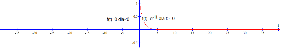
Fig. 6-1
The f(t) function
At first, f(t) looks like a single pulse of finite duration. But it lasts all the time from t=0 to t=+∞! We will treat f(t) as periodic with To=∞. But first as “really” periodic, that is, with a finite period To. We will calculate the Fourier Transform from Fourier Series. This approach, and not from a ready-made integral formula as Fig.6-15, will allow you to better understand the very idea of the Fourier Transform.
Chapter 6.2 Fourier series of the function f(t) with period To=15sec
Chapter 6.2.1 Graph of a function

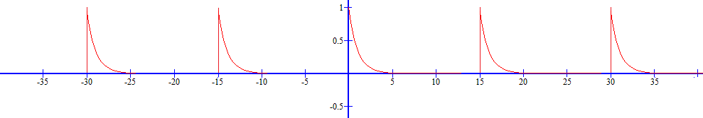
Fig. 6-2
Periodic function f(t) period To=15sec
That is, the first approximation of the f(t) function in Fig. 6-1. Why an approximation?
Because in the range e.g. t=-7.5…0…+7.5 sec you would only see the non-periodic function f(t) from Fig. 6-1!
Chapter 6.2.2 Reminder of the Complex Fourier Series formula
We will apply the general formula of the Fourier Series on c(n) in the complex version for positive and negative pulsations.
The constant component c(0), i.e. for n=0, also is valid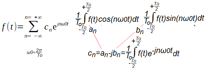
Fig.6-3
Complex formula for Fourier Series
The trigonometric formula for the Fourier Series is 2 separate formulas for a(n) and b(n).
Remember that the pulsation ω0 of the first harmonic is also the interval Δω between successive harmonics!
Chapter 6.2.3 Calculation of complex Fourier coefficients c(n) using WolframAlpha.
First harmonic pulsation–>ω0=2π/To=2π/15sec≈0.419/sec
Integration interval–>-To/2…+To/2=-7.5sec…+7.5sec.
For example, let’s calculate c(n) for n=+3.
WolframAlpha Instruction:
(1/15)*integrate exp(-t)*heaviside(t)*exp(-2pi*i*3*t/15)dx from t=-7.5 to 7.5 1
1. To implement it, copy the above text, i.e. cntrl c…
2.Click https://www.wolframalpha.com
3. Paste the text into the box.
4. Do what the picture says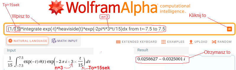

Fig.6-4
WolframAlpha instruction calculating the formula for c(n) in Fig.6-3 for n=+3, To=15 sec and f(t) in Fig.6-2
WolframAlfa also showed many other things, but we are only interested in the result, i.e. a complex number
c(+3)=c(+3ω0)=0.0259627-j0.0325001 for ω0=2π/15sec≈0.419*1/sec—>Fig.6-5.
This is the complex amplitude of the third harmonic, i.e. for ω=3ω0.
Chapter 6.2.4 Coefficients c(n) in the complex plane Re z/Im z
After calculations for n=-12…0…+12, I put the results of c(n) into the complex plane Re z/Im z. The complex Fourier coefficients c(n) will appear on the circle A. Among them is the one just calculated factor/point c(+3)=c(-3ω0)=0.0259627-j0.0325001. We also computed c(+1000)≈c(ω=-∞) and c(-1000)≈c(ω=+∞) as almost z=(0,0). In other words, n=1000 is as infinity.
Chapter 6.2.4 Coefficients c(n) in the complex plane Re z/Im z
After calculations for n=-12…0…+12, I put the results of c(n) into the complex plane Re z/Im z. The complex Fourier coefficients c(n) will appear on the circle A. Among them is the one just calculated factor/point c(+3)=c(-3ω0)=0.0259627-j0.0325001. We also computed c(+1000)≈c(ω=-∞) and c(-1000)≈c(ω=+∞) as almost z=(0,0). In other words, n=1000 is as infinity.

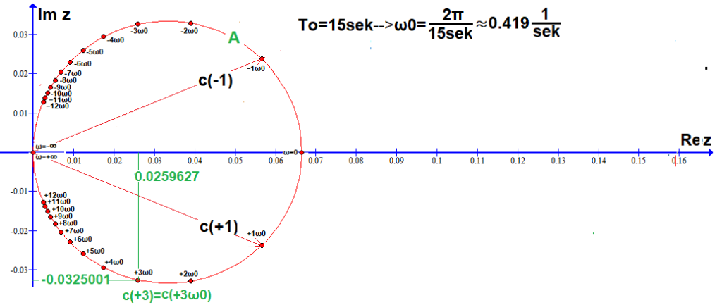
Fig. 6-5
26 Fourier Series c(n) coefficients on circle A calculated with the WolframAlpha program.
Including: bottom 12 c(n), top 12, c(ω=0), c(ω=+∞)=c(ω=-∞)=(0,0).
They form a lower semicircle for n>0, and an upper semicircle for n<0.
Each point c(n) for n=-12…+12 is the complex amplitude for the nth harmonic. So not exactly the nth harmonic.
I showed them as vectors only for c(+1)=c(+1ω0) and c(-1)=c(-1ω0). The remaining c(n) are just dots for readability.
The graph is the equivalent of the bar diagrams from chapters 3 and 4 concerning only even functions.
Conclusions:
1. c0=c(ω=0)≈0.0667-constant component when n=0
2. c(-∞)=c(+∞)=0+j0–>harmonics for ω=-∞ and ω=+∞ are infinitely small, let’s take them as zero.
3. c(+n)=c(-n)* are conjugate complex numbers, e.g. c(+1) and c(-1)*
4. Each c(n), i.e. the nth vector, corresponds to a harmonic with pulsation n*ω0, amplitude A i.e. vector length and phase φ.
E.g. c(+1)=c(+1*ω0) for ω0≈1*0.419/sec corresponds to the harmonic
h(+1)≈0.057*cos(0.419*t) -0024*sin(0.419*t)≈0.0307*cos(0.419*t-22.72°).
Similarly, the conjugate c(-1)=c(-1ω0) corresponds to the harmonic
h(-1)≈0.057*cos(0.419*t)+0024*sin(0.419*t)≈0.0307*cos(0.419*t+22.72°)
5. Points for n=-∞…-13 and n=+13…+∞ have not been marked. They thicken approaching z=(0,0) when ω=nω0–>+-∞.
Chapter. 6.2.5 Interpreting the graph in Fig.6-5 as Fourier Series
The 26 coefficients of c(n) in Fig.6-5 are nothing but the Fourier Series of f(t). Especially when you imagine that all the vectors are moving in circles around z=(0,0), each with its velocity +-nω0. The upper vectors are clockwise and the lower ones are opposite, as in the animation Fig. 6-6. Their sum as f(t) will always be on the real axis Re z, because they are formed by pairs of conjugate vectors, e.g. c(+1) and c(-1). So on the axis Re z there will be a projection of the sum of all rotating vectors, which will move as f(t) according to sum formula in Fig.6-3. This function f(t) will of course be from Fig.6-2, assuming n=-∞…0…+∞.
When n=-12…0…+12, such as in Fig. 6-2, f(t) will be “blunt”, otherwise without sharp points. These rotating vectors are a perfect example of a Complex Fourier Series formula.
The animation below shows counter-rotating 2 vectors whose sum, as f(t), moves only on the real axis Re z.

Fig.6-6
The sum of 2 oppositely rotating conjugate vectors
a-vector c(n)
b-conjugate vector, i.e. c(n)*
c-sum c(n)+c(n)*
Look again in Fig.6-3 for the ∑ pattern.
The real function f(t) is created by oppositely rotating pairs of vectors c(n)*exp(jnω0t) and c(-n)*exp(-jnω0t).
Chapter 6.2.6 Quotient Fourier Series, i.e. with coefficients c(n)/ω0
We divide each point/vector/coefficient c(n) in Fig.6-5 by ω0=Δω≈0.419*1/sec. In this way, it will be easier for us to go from Series to Fourier Transform. Similarly, we divided the amplitude a(n) by Δω in Fig. 4-2 in Chapter 4. The drawing is a bit large, but thanks to this the symbols +-1ω0,+-2ω0… are still legible.

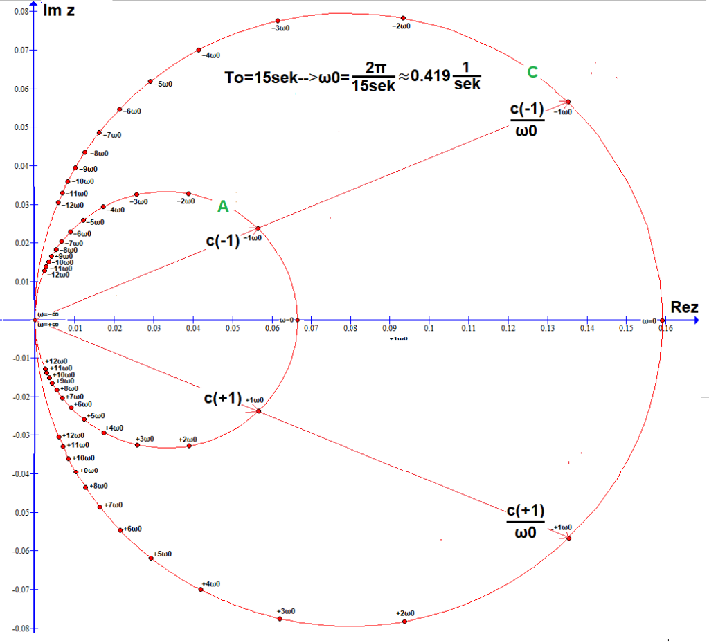
Fig.6-7
26 coefficients c(n) on circle A, i.e. repetition of Fig. 6-5.
26 coefficients c(n)/ω0 on circle C (ω0≈0.409)
Points c(n) on circle A have been transformed into points c(n)/ω0 on circle C. Why? Be patient.

Chap. 6.3 Fourier series of the function f(t) with period To=30sec
Chap. 6.3.1 Introduction
We will double the period To. The pulsation ω0=2π/30sec≈0.209/sec will be 2 times smaller than in chapter 6.2.
How will the corresponding coefficients/points c(n) and c(n)/ω0 in Fig.6-7 change?
Chapter 6.3.2 Time chart of a function f(t)

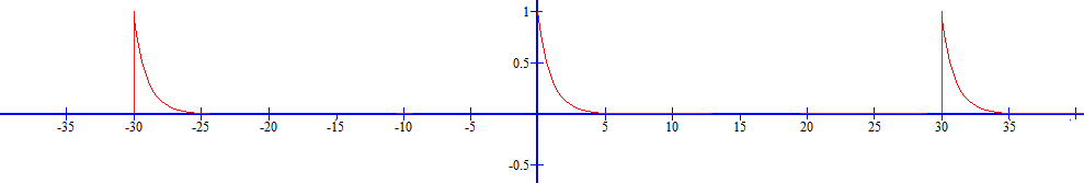
Fig. 6-8
Periodic function f(t) with To=30sec
This is the second and better approximation of f(t) in Fig. 6-1. Better, because To=30sec is closer to To=∞ than the previous one To=15sec. So we follow the path from chapter 3, in which we replaced a single rectangular pulse A=1 Tp=1sec with a sequence of these pulses, i.e. periodic functions with an increasing period To.
Chapter 6.3.3 Calculation of complex Fourier coefficients c(n) using WolframAlpha
We will calculate the Fourier coefficients c(n) in the same way as in Chapter 6.2.
The instruction for WolframAlpha for e.g. n=3 will be:
(1/30)*integrate exp(-t)*heavisde(t)*exp(-2pi*i*3*t/30)dx from t=-15 to15
Chapter 6.3.4 Coefficients c(n) in the complex plane Re z/Im z

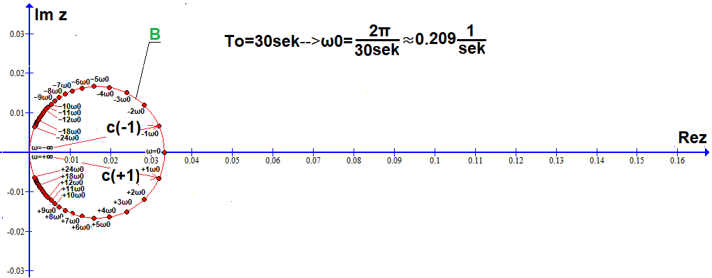
Fig.6-9
50 coefficients c(n) of the Fourier Series on circle B calculated with the WolframAlpha program.
Including:
24 lower c(n),24 upper c(n), c(ω=0), c(ω=+∞)=c(ω=-∞)=(0,0).
Compare with Fig.6-5 when To=15sec.
Conclusions:
The coefficients c(n) are smaller and more densely distributed on circle B twice smaller than A, because the intervals Δω=ω0≈0.209/sec between successive harmonics are twice smaller. What if the vectors started rotating around z=(0.0)? Then the projection of the sum of these vectors would move along the Re z axis similarly to f(t) from Fig. 6-8, only in a “more smooth and no peaks” way.
Chapter 6.3.5 Quotient Fourier Series, i.e. with coefficients c(n)/ω0
We divide each c(n) in Fig. 6-9 by ω0=Δω≈0.209*1/sec.

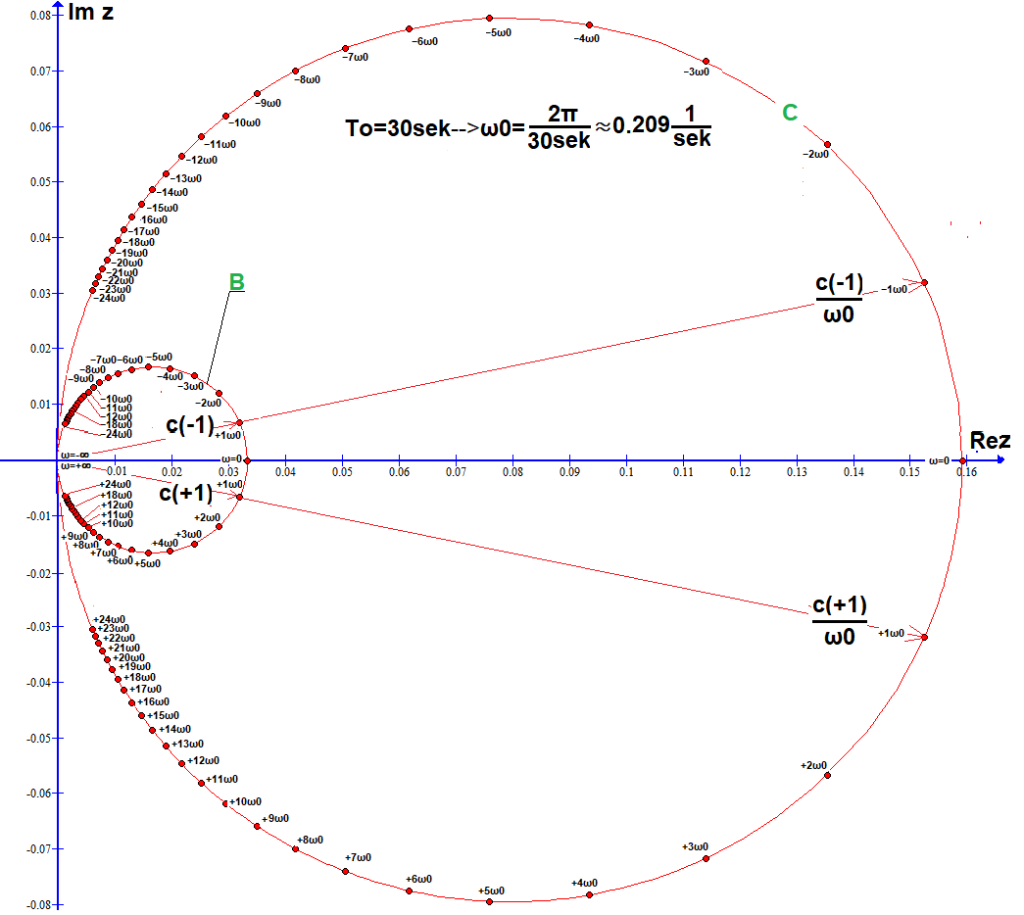
Fig.6-10
50 c(n) coefficients on circle B and 50 c(n)/ω0 coefficients on circle C (ω0≈0.209/sec)
Circle B is 2 times smaller than A in Fig. 6-5 and Fig. 6-7 and the coefficients c(n) are twice as densely distributed.
The circle C is the same as in Fig. 6-7, only the coefficients c(n)/ω0 are twice as densely distributed.

Chapter 6.4 What happens when It increases, i.e. ω0 decreases?
Chapter 6.4.1 Introduction
In chapter 6.2 was To=15sec and in 6.3 it increased to To=30sec. What effect did this have on the coefficients c(n)?
Chapter 6.4.2 Comparison of 2 graphs
So Fig. 6-7 and Fig. 6-10 on one collective. The drawing has a larger scale and therefore the circles A,B,C are now smaller. For some reason, I added a circle D, which is a circle C enlarged by 2π times. The points c(+1)/ω0 and 2π*c(-1)/ω0 on C and D are presented as vectors. The other points on the circles are also vectors, of course.

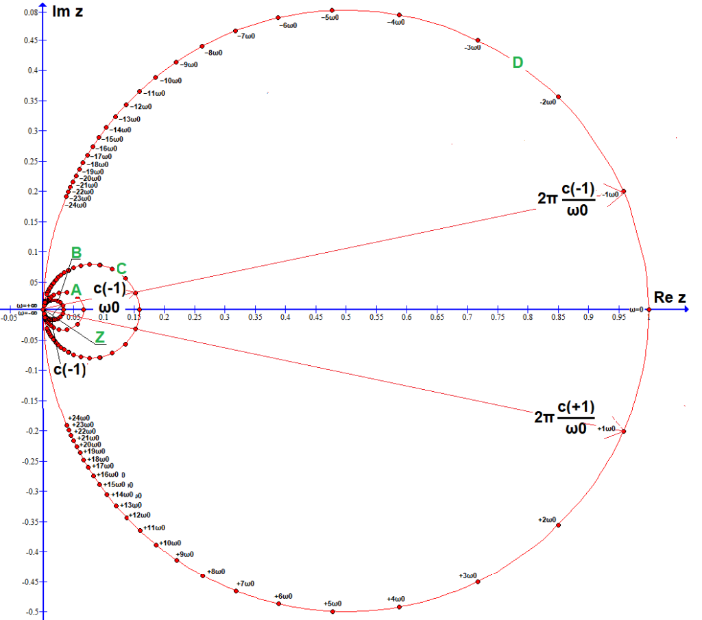
Fig. 6-11
Complex coefficients c(n), c(n)/ω0 and 2π*c(n)/ω0 on circles A,B,C,D and the mysterious “point-circle” Z adjacent to (0,0).
–circle A with 26 points c(n) from Fig.6-5 when ω0=0.409 (To=15sec)
–circle B with 50 points c(n) from Fig.6-9 when ω0=0.209 (To=30sec)
–circle C with “quotient” points c(n)/ω0 from Fig.6-10:
with 26 points c(n) when ω0≈0.409 (To=15sec)
with 50 points c(n) when ω0≈0.209 (To=30sec)
Note:
Although circle B is 2 times smaller than A, its c(n) has been divided by 2 times smaller ω0.
Therefore, all points c(n)/ω0 from A and B are on the same circle C.
-circle D with points 2π*c(n)/ω0, i.e. circle C magnified by 2π
with 26 points c(n) when ω0≈0.409 (To=15sec)
with 50 “quotient” points c(n) when ω0≈0.209 (To=30sec)
Why 2π magnification? We’ll find out later. For now, “to see better”.
All points on circles C and D come from B, but only every second one from A. If the vectors on circles A and B started to rotate with velocities n*ω0, their projections onto the real axis Re Z would be similar to f(t) from Fig. 6-2 and 6-8, only more blunt and “tipless”.
Chapter.6.4.3 It’s still growing…
We analyze the function f(t) similar to Fig.6-8, only “rare” because To=60sec. What would change in Figure 6-11?
1. Inside C there would be a circle E 2 times smaller than
Note:
Circle E and its f(t) are not shown in the figures.
2. Circle E contains 2*48+1+1=98 points/coefficients c(n)
3. There would be 98 “descendants” of E in circles C and D. Similar to 50 “descendants” of B in C and D in Fig. 6-11
Conclusion
As To increases, smaller and smaller circles A,B,E,F,G…Z are formed with c(n) points getting closer to each other. Compare, for example, A and B. Clearly points c(n) on B are “denser”. Not only because B is smaller than A! Also because the distance Δω0=ω0 between c(n) has decreased twice. These diminishing circles A,B,E,F,G…Z become more and more “continuous”. Until there is an infinitely small and continuous circle Z when To=∞. It is the previously mentioned mysterious “point-circle” Z in Fig.6-11. Here the spacing between points/vectors c(n)=c(n*dω) is infinitely small (To–> ∞ i.e. dω=ω0–>0).

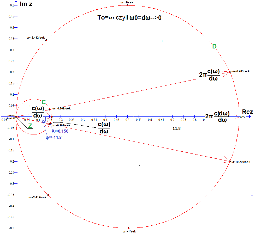
Rys. 6-12
Okręgi C i D oraz nieskończenie mały okrąg Z wewnątrz C
Te “dotykające” się punkty c(n), na nieskończenie małym i ciągłym okręgu Z są współczynnikami Szeregu Fouriera nieokresowej funkcji f(t) z Rys.6-1. Tzn. istnieje harmoniczna dla każdej ciągłej pulsacji ω, a nie tylko dla konkretnych ω=n*ω0 jak na Rys.6-7 i 6-10. Inna rzecz, że każda harmoniczna jest nieskończenie mała! Trudno coś tak małego jak Z analizować. Jeżeli współczynniki c(n) na okręgach A, B, E,…podzielisz przez odstęp Δω=ω0 między nimi (dla A–>Δω=ω0≈0.419/sek, dla B–>Δω=ω0≈0.209/sek), to punkty c(n)/ω0 znajdą się na tym samym okręgu C. Czyli okręg C o współrzędnych c(ω)/dω, to powiększone (“przez lupkę”) punkty c(ω) okręgu Z. Zaś okrąg D jako 2π*c(ω)/dω, czyli powiększony 2π razy okrąg C, jak się później okaże, jest właśnie transformatą funkcji f(t) z Rys. 6-1.

Chapter 6.5 What is the Fourier Transform of f(t) in Fig. 6-1?
Chapter 6.5.1 Introduction

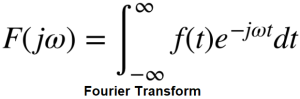
Fig. 6-13
Fourier transform
Most authors start with this. It doesn’t say what a Fourier Transform is, but how it is computed. It’s as if someone defined a hammer as a product that needs to be made in a certain way. And it should be. A hammer is a tool for driving nails. And the Fourier Transform is a formula that allows you to calculate the distribution of harmonics in the f(t) signal.
Chapter 6.5.2 What is the circle C with coordinates c(ω)/dω in Fig.6-12?
The infinitesimal circle Z consists of points c(ω), each of which is a vector corresponding to a harmonic with ω pulsation.
For example, for pulsation ω=+1/sec, it is a harmonic with infinitely small amplitude A and phase φ≈-11.8º. For now, take my word for it, especially when it comes to φ=-11.8º. But if you enlarge Z by operation c(ω)/dω, you will get circle C in Fig.6-12, where “you can see more”, also φ≈-11.8º. From this it follows that the amplitude A of the harmonic with pulsation, e.g. ω=+0.209/sec of the function, although infinitely small, is greater than that when ω=+1/sec and smaller than ω=0/sec. And the expression c(ω)/dω itself is the harmonic density with respect to the ω pulsation. Just as the mass of lead at point is zero m=0, but its density relative to volume V is isn’t zero ρ=11.34 g/cm³! Considering that we are dealing with the vector c(ω)/dω, treat the density of this vector for ω=+0.209/sec as its average value around the pulsation ω=+0.209/sec. So we sum/integrate all (infinitely small!) vectors, e.g. for ω=+0.2085/sec…ω=+0.2095/sec and divide by Δω=0.2095/sec-0.2085/sec=0.001sec. The result is the vector c(ω)/Δω≈0.156*exp(-j11.8º). So the spectral density of the exponential function f(t) from Fig. 6-1 for ω=+0.209/sec is a vector with amplitude A=0.156 and phase φ≈-11.8º. And translating into harmonics, f(t) from Fig. 6-1 has a harmonic around ω=+0.209/sec with an average value of h(t)=0.156*cos(0.209t-11.8º). Needless to say, the value of c(ω)/dω is most accurate when Δω–>dω–>0. Just like the mass density at the point ρ=m/Δv is the most accurate when Δv–>0.
Coming back to the question in Chapter 6.5.1. Circle C is “almost” a transform of the f(t) from Fig.6-1. And “not almost” but “exactly”, then the Fourier Transform of the function f(t) is the circle D in Fig. 6-12.
Why? See Chapter 6.5.3.
Chapter 6.5.3 More about the Fourier Transform
You already know that the Fourier Transform of f(t) is the complex function F(jω) in the form of a circle D in Fig. 6-13. And other functions, more precisely those whose area under the function f(t) is finite? That is, any, although not entirely. Imagine that this is a slightly different function than f(t) in Fig. 6-1, but non-periodic and with a finite area. However, it cannot be e.g. f(t)=exp(t).

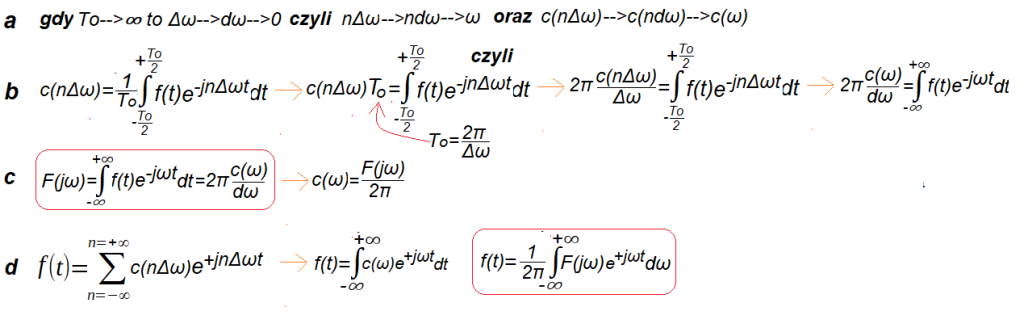
Fig. 6-14
a. What happens when the period To of f(t) approaches infinity?
Then the first harmonic ω0=Δω tends to the infinitely small dω. This also means that the intervals dω between successive harmonics are infinitely small. In other words, successive harmonics “overlap” and their distribution c(n*dω) becomes continuous c(ω).
b. c(nΔ) is the nth complex amplitude when f(t) is a periodic approximation f(t) for finite To.
When To=∞ then c(ω)/dω becomes continuous and 2π*c(ω)/dω is just the Fourier Transform F(jω) of f(t)!
c. The final formula for the Fourier transform of F(jω). Note that it is c(ω)/dω augmented by 2π.
d. When the non-periodic f(t) approximation is periodic (with a long period To!), then f(t) is the usual Fourier Series formula on the left. And when To–>∞ the formula for the Fourier Series becomes a continuous formula for the so-called Inverse Fourier Transform. It allows you to calculate the waveform f(t) based on its Fourier Transform F(jω).
Chapter 6.6 Fourier Transform and Inverse Fourier Transform.
That is the final summary of the chapter

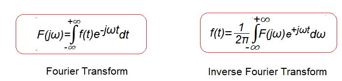
Fig. 6-15
Fourier Transform and Inverse Fourier Transform
One of the most famous pairs of mathematical equations. It is good to know them, even if they are not fully understood.