3. Fourier Transform of a single square wave pulse part 1

Fourier Transform

Chapter 3 Fourier Transform of a single square wave pulse part 1
Chapter.3.1 Introduction
It is difficult to find a simpler non-periodic function f(t) than a single rectangular pulse in Fig. 3-1a. It is an even function with amplitude A=1 and duration Tp=1sec. The Fourier Transform is generally a complex function. But thanks to the even of f(t), its Fourier Transform F(ω) is also a real function. And this one is easier to analyze than the complex function. Let me remind you that every real function and real number is complex, but not vice versa! Due to the length, the topic has been divided into chapters 3 and 4.

Chapter 3.2 A single square wave pulse as a signal with an infinite period To=∞.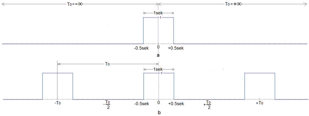

Fig. 3-1
a. Single rectangular pulse
– amplitude A=1
– duration Tp=1sec
The impulse is an even function.
b. Periodic function as a sequence of pulses with period To, duration Tp=1sec and amplitude A=1.
A single rectangular pulse as a, can be treated as a periodic function b with infinite period To=∞.

Chapter 3.3 Square waves with increasing period To.
We will examine several square waves of different To but with the same amplitude A=1 and duration Tp=sec.

Fig.3-2
Periodic functions with pulse A=1, Tp=1sec and increasing period To.
a. To=2 sec –>ωo=1π/sec
b. To=4 sec–>ωo=1π/2sec
c. To=8 sec–>ωo=1π/4sec
d. To=16 sec–>ωo=1π/8sec
Waves 2, 4, 8, 16 sec are increasingly similar to a single pulse. And the most is To=16sec. So we can calculate the Fourier coefficients a(n) for this wave from the known formulas and say that we have “almost” decomposed the “single” f(t) from Fig.6-1a into harmonics.
Note:
The pulses should be synchronized. They are “almost” in the animation. Sorry.

Chapter.3.4 What formula will we use for bar diagrams?
The bar diagrams applies only to even functions and is the most intuitive version of the Fourier Series. We will examine the effect of the increasing period To of Fig. 3-2 on the bar diagrams . This will make it easier for us to understand the idea of the Fourier Transform as a “descendant” of the Fourier Series. We will start with the general trigonometric formula.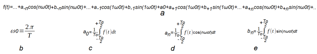

Fig. 3-3
Trigonometric Fourier formula for any function f(t) with period To.
In the complex version c(n)=a(n)-jb(n).
Note:
The interval of integration in formulas c,d,e is -To/2…+To/2. It can also be different, e.g. 0…To or -To/4…+To3/4,
provided that its length is To. For the even function f(t) there are no b(n) components and the formula will simplify.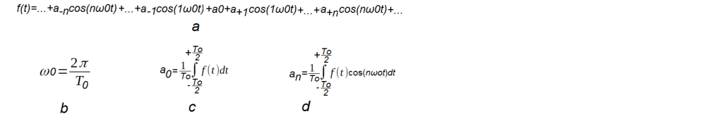

Fig. 3-4
Trigonometric Fourier Series formula for an even periodic function f(t).
All bar diagrams, animations in this and the next chapter will be related to the above formula. We will specialize it even more for a square wave f(t) with duration Tp=1sec and amplitude A=1. It pays off because there will be a lot of repetitive calculations. The period of the wave To increases from 2 sec to ∞ with a constant pulse duration Tp=1sec. So the duty cycle decreases from 50% to 0%.

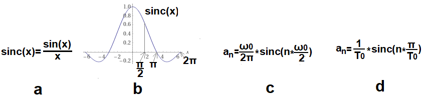
Fig. 3-5
Fourier Series formulas for the square wave in Fig. 3-1b for different To, that is different ω0=2π/To.
Derivation of the formulas in Fig. 3-11.
They apply to square waves in which:
– rectangular pulse has a constant value A=1 and Tp=1sec.
– only the period of occurrence of these pulses To increases.
Thanks to them, we can easily determine the coefficients a(n) necessary for the animation of bar diagrams.
a. Definition of the sinc(x) function.
The function f(x)=sin(x)/x appears so often in signal theory that a special name sinc(x) was created for it. Note that although every period T=πsec the function resets to 0, it is not periodic! It tends to 0 when x–>+/-∞ and sinc(0)=1 is its maximum. It’s a bit weird at first because we’re dividing by 0! But there is a “0/0” –> de l’Hospital’s rule and everything is lege artis.
b. The sinc(x) function graph
Characteristic points x=0,π/2, π and 2π are shown.
The chart shows, for example, that:
– sinc(0)=1
– sinc(π/2)=2/π≈0.637
– sinc(1π)=sinc(2π)=…sinc(nπ)=0
– sinc(+∞)= sinc(-∞)=0
c. Formula for a(n) as a function of ω0 pulsation. There is the amplitude of the nth harmonic for the n*ω0 pulsation, where ω0 is the pulsation of the periodic function f(t).
d. The formula for a(n) as a function of period To. It is also the amplitude of the nth harmonic for the period To/n, where To is the period of the periodic function f(t). We will use this formula most often. Recall that ω0=2π/To.
For example, let’s calculate a1(ω0=1π/sec)=a1(To=2sec). That is, the first harmonic for the square wave in Fig. 3-2a.
We will use the 3-5d formula
a(1)=(1/2)*sinc(1*π/2)=1/π≈0.318
We used the plot of Fig. 3-5b, where sinc(π/2)=2/π≈0.637
Note
1. Formulas are valid for n=-∞…0…+∞. For n=0, the harmonic is the constant component a(0).
2. They come from the integral formula Fig.3-4d.
For doubters – derivation in chapter 3.5.7

Chapter 3.5 Bar diagrams for periodic functions
More precisely for periodic functions a, b, c and d from Fig. 3-2.
Chapter 3.5.1 Introduction
Recall the 4 animations from Fig. 3-2.
Each of them is:
-even function of time f(t)
-a square wave consisting of square pulses Tp=1sec repeating every period To.
-the first pulse begins during half of its duration Tp=1sec and therefore f(t) is an even function.
We will examine the effect of increasing period To on the bar diagrams. We will use the formula Fig. 3-5d. It was assumed that A=1 and Tp=1sec. Therefore, the only variables in the formula Fig. 3-5d are To as the period of the first harmonic of the function and n as the nth harmonic.
Chapter 3.5.2 Bar diagram for wave A=1, Tp=1sec and To=2sec
For the first wave f(t), i.e. for Fig. 3-2a, we have already made a bar diagram in subchapter 2.4 chapter 2. This is a typical square wave with amplitude A=1 and period To=2sec. Its duty cycle is 1/2. In the formula of Fig.3-5d, the only variable is n because the period of the wave is constant To=2sec. It corresponds to the pulsation ω0=1π/sec.
Let’s calculate a(-n)=a(+n) for n=0…3. and To=2sec according to the formula Fig. 3-5d.
n=0–>ω=0*ω0=0
a(0)=(1/2)sinc*(0*π/2)=1/2=0.5 bo sinc(0)=1 acc. Fig. 3-5b
n=1–>ω=1*ω0=1π/sek
a(-1)=a(+1)=(1/2*)sinc(1*π/2)=1/(2π)≈0.318
n=2–>ω=2*ω0=2π/sek
a(-2)=a(+2)=(1/2)*sinc(2*π/2)=0
n=3–>ω=3*ω0=3π/sek
a(-3)=a(+3)=(1/2)*sinc(3*π/2)=-1/(3*2π)≈-0.106
Note
You can check the above data with WolframAlfa. How? See Chapter 11.2 WolframAlpha program of the article “Rotating Fourier Series” from the top tab.
E.g. To calculate a(-3)=a(+3) call WolframAlfa
Click https://www.wolframalpha.com
Then type or paste into thewindow 0.5*sinc(3*pi/2) and do what the picture says.

Fig. 3-6
The program correctly calculated a(-3)=a(+3)=(1/2)sinc(3*π/2)=-1/3π≈-0.106103.

Fig. 3-7
Square wave bar diagram A=1, Tp=1sec, To=2sec from Fig. 3-2a
That is, for the first wave f(t) in Fig. 3-2a with 1/2 duty cycle.
The state of harmonics before the animation, i.e. in the initial state, i.e. for t=0. What does the picture show?
1. Non-pulsating DC component a0=0.5
2. First harmonic pulsations 1ω0=+1π/sec and -1ω0=-1π/sec
3. There are only odd harmonics +-1*π/sec, +-3*π/sec, +-5*π/sec…
4. Coefficients a(+1), a(-1), a(+3), a(-3) are the amplitudes of +0.318, -0.106 of the pulsating bars. For example, negative -0.106 means that this was the value of the 3rd harmonic in the initial state for t=0.
5. Only 4 harmonics and component a0=+0.5 are shown. Other i.e. for ω=-∞…-5π/sec and ω=+5π/sec…+∞ are invisible.
6. Invisible harmonics, however, are included in the pulsating bar f(t). It is the sum of all harmonics, invisible too! Note that this is a perfect square wave. No “waves”, i.e. without the Gibbs effect.
7. A square wave as a pulsating line f(t) is in phase with the first harmonic.
8. f(t)=…-(1/3π)*cos(3π*t)+(1/1π)*cos(1π*t)+0.5++(1/1π)*cos(1π* t)-(1/3π)*cos(3π*t)…
The bar diagram animation and the above equation represent exactly the same thing. The f(t) function is a vertical line appearing every To= 2sec, i.e. with a pulsation of 1ω0=+1π/sec. You see the harmonics in equation 8 as pulsating bars with ω=-3π/sec, ω=-1π/sec, ω=0, ω=+1π/sec, ω=+3π/sec. The remaining harmonics are invisible, but included in the total on f(t). That’s why you see the f(t) band as perfect jumps every To=2sec.
Chapter 3.5.3 Bar diagram for wave A=1, Tp=1sec and To=4sec
That is, for the second wave f(t) in Fig. 3-2b with 1/4 duty cycle.

Chapter 3.5.3 Bar diagram for wave A=1, Tp=1sec and To=4sec
That is, for the second wave f(t) in Fig. 3-2b with 1/4 duty cycle.

Fig. 3-8
Square wave bar diagram A=1, Tp=1sec, To=4sec–>ω0=π/2sec from Fig. 3-2b
Let’s calculate a(-n)=a(+n) for n=0…6 according to formula Fig. 3-5d.
n=0–>ω=0*ω0=0
a(0)=(1/4*)sinc(0*π/4)=(1/4)*1=1/4=0.25
n=1–>ω=1*ω0=1*π/2sek
a(-1)=a(+1)=(1/4)sinc(1*π/4)≈0.225
n=2–>ω=2*ω0=2*π/2sek=1*π/sek
a(-2)=a(+2)=(1/4)*sinc(2*π/4)≈0.159
n=3–>ω=3*ω0=3*π/2sek
a(-3)=a(+3)=(1/4)*sinc(3*π/4)≈0.159
n=4–>ω=4*ω0=4*π/2sek=2*π/sek
a(-4)=a(+4)=(1/4)*sinc(4*π/4)=0
n=5–>ω=5*ω0=5*π/2sek
a(-5)=a(+5)=(1/4)*sinc(5*π/4)≈-0.045
n=6–>ω=5*ω0=6*π/2sek=3*π/sek
a(-6)=a(+6)=(1/4)*sinc(6*π/4)≈-0.053
Conclusions
1.The DC component a0 and the harmonic amplitudes are 2 times smaller than for the previous square wave in Fig. 3-2b. This agrees with intuition, because a rectangular pulse is 2 times less frequent.
2.The envelope of the pulsating bars is also 2 times smaller vertically. This follows from the formula Fig. 3-5d. This means that the zero points of ω=1π, 2π, 3π…are the same. This, of course, applies to all square waves in Fig. 3-2.
3.The bars are twice as densely spaced. This also follows from the formula Fig. 3-5d, but I will try to support it with intuition. It’s probably harder to choose the cosines so that they add up to a pulse that occurs less often! The job needs to be more subtle. i.e. harmonics are not only 2 times smaller, but there are 2 times more of them. Just like with more Lego bricks, but smaller and more complicated, you can build a more complicated car. This “rarer impulse” is a more complicated car.
4.Pay attention to the less frequent impulse A=1 Tp=1sec.
Chapter 3.5.4 Bar diagram for wave A=1, Tp=1sec and To=8sec
That is, for the third wave f(t) in Fig. 3-2c with 1/8 duty cycle.

Fig. 3-9
Square wave bar diagram A=1, Tp=1sec, To=4sec–>ω0=π/2sec from Fig. 3-2c
Let’s calculate a(-n)=a(+n) for n=0…12 according to formula Fig. 3-5d.
n=0–>ω=0*ω0=0
a(0)=(1/8)*sinc(0*π/8)=1/8=0.125
.
.
n=12–>ω=12*ω0=3*π
a(12)=(1/8)*sinc(12*π/8)≈-0.026
I gave only 2 calculations, you can calculate the rest with WolframAlfa program.
The pulse f(t) occurs every To=8 sec.
Chapter 3.5.5 Bar diagram for wave A=1, Tp=1sec and To=16sec
That is, for the fourth wave f(t) in Fig. 3-2d with 1/16 duty cycle.
Chapter 3.5.5 Bar diagram for wave A=1, Tp=1sec and To=16sec
That is, for the fourth wave f(t) in Fig. 3-2d with 1/16 duty cycle.

Fig. 3-10
Square wave bar diagram A=1, Tp=1sec, To=16sec–>ω0=π/8sec from Fig. 3-2d
Let’s calculate a(-n)=a(+n) for n=0…24 according to formula Fig. 3-5d.
n=0–>ω=0*ω0=0
a(0)=(1/16)* sinc(0*π/16)=1/16=0.0625
…
…
n=24–>ω=24*ω0=3*π
a(24)=(1/16)*sinc(24*π/16)≈-0.013
The pulse f(t) occurs every To=16 sec.
I emphasize again.
The bar diagram, and especially its animation, is the most intuitive representation of a Fourier Series. You can see what you can’t see in the formula Fig.3-4. i.e. mutual correlation between successive harmonics as in Fig. 3-10. And animation is already a cosmos! You can see the f(t)-left side of the Fourier Series as a sum of swinging bars. The function f(t) is an impulse A=1, Tp=1sec appearing as a vertical line every To=16sec.
Chapter 3.5.6 Effect of increasing To period on the bar diagram.
In Fig. 3-2, the pulse has a constant amplitude A=1 and duration Tp=1sec. The period To of the square wave increases. The impulse becomes more and more solitary, gradually resembling a single impulse. On ordinary, read static, diagrams, this is not visible, but on animations it is.
Let’s get back to the conclusions, so what happens to the bars when the period To increases? Recall that the nth bar is the nth harmonic. You see only the most important initial bars in the range. The others, invisible and tending to zero, you have to imagine.
Conclusions
1. The bars are more and more densely located
2. The envelope of the bars flattens out.
3. Zeros ω=…-3π,-2π,-1π,0,+1π,+2π,+3π…are constant.
4. Max 1/2.1/4.1/8.1/16 correspond to ω=0 bars, i.e. the constant component a(0) of the Fourier Series of square waves from Fig. 3-2a,b,c,d.
5. The sum of all bars-harmonics is a function of f(t) and appears every 2, 4, 8 or 16 seconds as a vertical line – a perfect square wave.
Chapter 3.5.7 Derivation of the formula for volunteers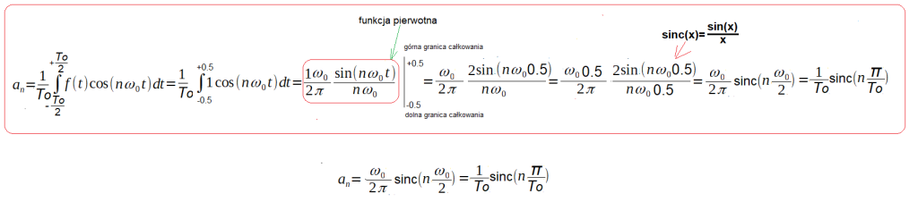

Fig. 3-11
Derivation of the Fourier Series formula for the wave from Fig. 3-1b
This is a highly specialized function f(t) and applies only to a sequence of pulses with amplitude A=1 and duration Tp=1sec. Only the period of the function To (or the pulsation ωo) and n changes. The ωo pulsation concerns the first harmonic and is also the distance Δω=ω0 between the bars. Basic knowledge of calculus is enough. The formula is also valid for the constant component–> n=0.