4. Fourier Transform of a single square wave pulse part 2

Fourier Transform

Chapter 4 Fourier Transform of a single square wave pulse part 2
Chapter 4.1 Fourier series of rectangular pulse trains A=1 Tp=1sec with increasing period To.

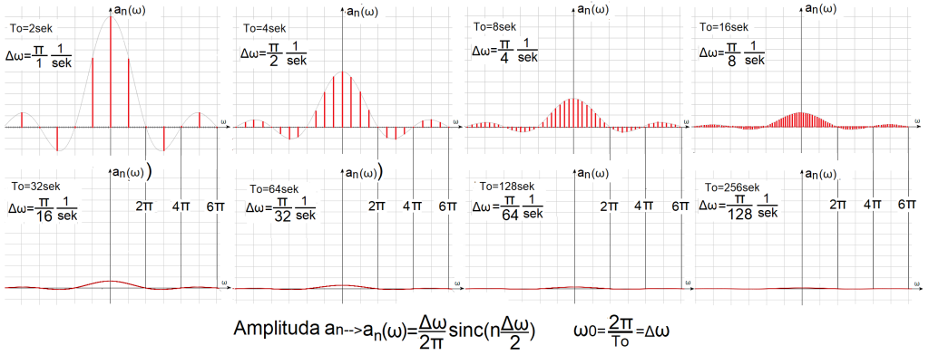
Fig. 4-1
Fourier series of sequences of rectangular pulses A=1 Tp=1sec as bar diagrams.
This is a graphical summary of the chapter 3, in which the pulses A=1 T=1sec become increasingly rare. The formula for the a(n), the amplitude of the nth harmonic, and the bar diagram represent the same thing. The upper bars were swinging in chapter 3 as animations in Fig. 3-7…10. The largest bars are the middle constant components a(0). The first right bars from a(0) are a(+1) and the first left ones are a(-1) and refer to the first harmonics for +,- pulsations. The lower bars are already so dense that they look like red envelopes.
Conclusions:
The “upper left” harmonic distribution for waves with period To=2sec and pulse A=1, Tp=1sec (i.e. dense pulses), consists of sparsely distributed harmonics with large amplitudes a(n).
The “lower right” harmonic distribution for waves with period To=256sec and pulse A=1,Tp=1sec (i.e. rare pulses), consists of densely distributed harmonics with small amplitudes a(n).
And what would a square wave with an infinite period To and an impulse A=1 and Tp=1sec, i.e. a single impulse, consist of? On the feel, these will be infinitesimal harmonics a(n) with infinitely little different pulsations Δω->dω–>0. So the discrete formula for the amplitude an of the next harmonic an=a(n*Δω) will become a continuous function a=a(ω). Each ω pulsation will be assigned some amplitude, and not only for ω=n*Δω pulsations. Another thing is that the amplitudes are then infinitely small, but not zero! The closest to such a situation is the bar diagram for To=256 sec. Here It is “almost” infinity. These increasingly flat graphs of a(n*Δω) want to tell us something, but what? The answer to such questions is the Fourier Transform, used to study the harmonics of a single pulse, and generally non-periodic functions.
Chapter 4.2 How to go from Fourier Series to Fourier Transform?
For now, the transform only for a specific single pulse.
Fig. 4-1 shows that the bar diagrams become:
–more dense
-the intervals between successive a(n) are getting smaller
–more “flat”
So divide an(ω) from Fig. 4-1 by Δω, you get the quotient version. The “flat” defect will disappear and subsequent bar diagrams will look like this. The value of ω becomes continuous when Δω–>dω–>0 ω=n*dω. Because then for every continuous ω there are n and dω such that ω=n*dω.

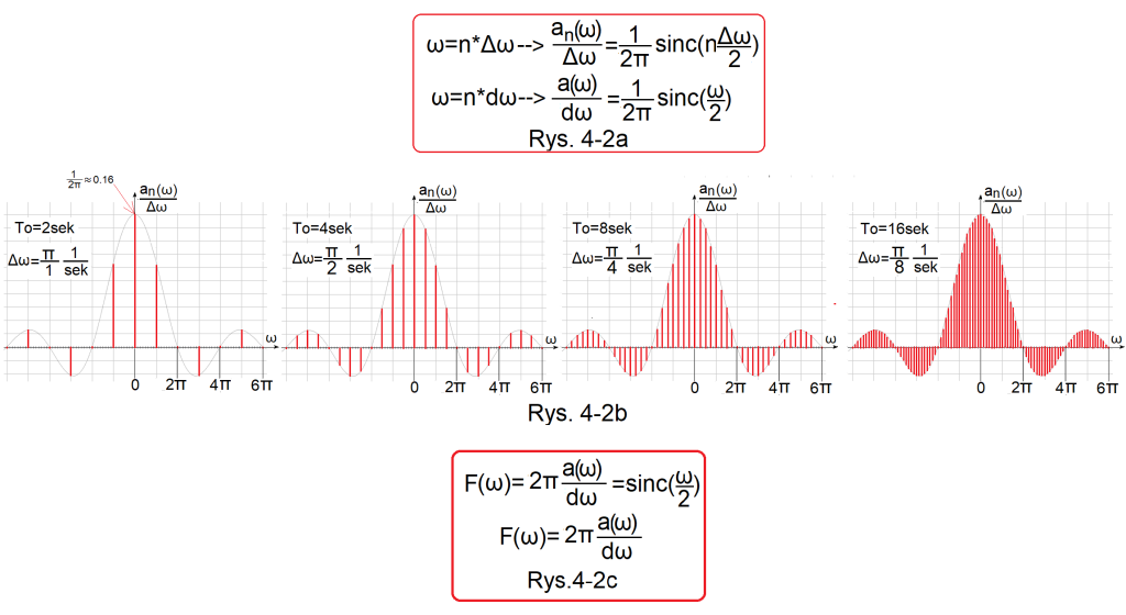
Fig. 4-2
Quotien version of the Fourier Series of a square wave for decreasing spacing Δω
Fig. 4-2a
The quotient an(ω)/Δω, when Δω is a specific finite value, is a discrete function, i.e. it exists only for specific ω=n*Δω.
The quotient an(ω)/dω, when dω is infinitely small, is a continuous function, i.e. it exists for any ω. For every n and dω there is an arbitrary (continuous) ω such that ω=n*dω.Fig. Fig.4-2b
The results of the next 4 “quotient” versions of the Fourier Series of square waves in the bar diagrams.
Quotients an(ω)/Δω for f(t) pulse A=1, Tp=1sec with increasing periods To=2, 4, 8 and 16 sec.
Fig. 4-2c
This is actually a repetition of Fig. 4-2a, where the transform F(ω) of a single rectangular pulse x(t) is defined as the amplitude density a(ω) with respect to the pulsation ω (multiplied by 2π). Here x(t) is a single rectangular pulse “starting” in its center–>Fig.3-1a, but this applies to all single pulses x(t) being even functions. In chapter 5 we will generalize this formula to all x(t) functions, not necessarily even ones.
Conclusions:
1. The envelope of each plot is the same! i.e. its maximum a0/ω0=1/2π≈0.16 and zeros ω=0,+/-2π,+/-4π,+/-6π… are the same for each series. “Something like that” is easier to analyze than the increasingly flat amplitudes in Fig. 4-1.
2. The subsequent “quotient” Fourier Series are “denser”, because the intervals Δω=ω0 between successive amplitudes a(n) and a(n+1) decrease.
3. Equivalents of the bottom 4–>”flat” from Fig.4-1 you have to imagine. They will be similar to Fig.4-2a, only more “dense”.
4. And now the most important thing. The above “quotient” versions, let’s call them an/Δω, are discrete, otherwise discontinuous functions. So they exist only for ω=n*Δω and not for any ω! And when will they become continuous functions? So the envelope of these bar diagrams? Then when Δω becomes infinitely small, i.e. when Δω–>dω as in Fig.4-2a.

Chapter 4.3 Interpretation of the Fourier Transform F(ω) for a pulse f(t)=A=1 Tp=1sec
Because it’s the easiest for this particular f(t) function. All its harmonics start in the same phase φ=0 e.g. for ω=1π/sec or φ=-180º e.g. for ω=1π/sec–>Fig.4-3c. Therefore, classical f(x) bar diagrams can be used, which cannot be said for any impulse whose harmonics have different initial phases φ. We will talk about such transforms in Chapter 5.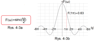

Fig. 4-3
Transform F(ω) of a rectangular pulse A=1 and Tp=1sec (“starting in the middle”)
Fig. 4-3a
Transform F(ω)
Fig. 4-3b
Bar diagram F(ω) of this transform
How to treat him? E.g. F(ω=1π/sec)≈0.63. Does this mean that for ω=1π/sec, the amplitude of this harmonic is 0.63? Nooo! After all, this impulse consists of infinitely small harmonics infinitely little differing in pulsation. So the harmonic A(ω=1π/sec)=0. But the sum/integral of these harmonics in a small range, e.g. Δω=0.9999π…1.0001π will no longer be zero!

Chapter 4.4 What is the Fourier Transform?
Chapter 4.4.1 Introduction
1. The transform is information about the frequency distribution in a given signal.
2. So it is a function of the pulsation F(ω).
3. It is mostly a complex function F(ω). This will be discussed in Chapter 5. Fortunately, our impulse A=1, Tp=1sec is an even function, and the transforms of even functions are “easier”, because they are real F(ω) functions. Therefore, we can present it in the form of the formula Fig.4-3a or the bar diagram Fig.4-3b.
Chapter 4.4.2 Rod and transform
Analogies will make it easier to understand the idea of the transform.
In particular, the harmonic A(ω) for ω is zero, but the transform F(ω) for ω is non-zero.

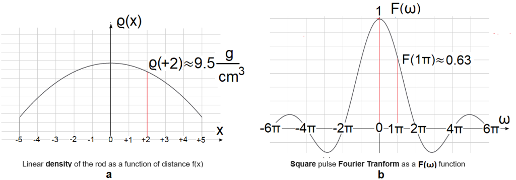
Fig.4-4
Rod specific density ϱ(x) and square wave transform F(ω) analogy.
Fig.4-4a
Rod specific density as a distance function ϱ(x)
The mass of the rod in any cross-section x is zero because the volume of each cross-section is ΔV=0.
The rod density ϱ(x) in any x-section is not zero. A lead-aluminum alloy rod with a cross-section of s=1cm2 and a length of l=10m. The density of the rod is the smallest at the ends of -5m +5m and the highest in the middle. In other words, there is only aluminum at the ends, only lead in the middle, and an alloy with an intermediate composition in the rest. E.g. ϱ(x=+2)≈9.5g/cm3
Fig.4-4b
Square pulse transform as a function of pulsation F(ω)
The amplitude of the harmonic A(ω) for any ω pulsation is infinitely small, let us assume that it is zero.
The amplitude density with respect to ω, i.e. “almost” the F(ω) transform, because F(ω)=2π*a(ω)/dω is non-zero. E.g. F(1π/sec)≈0.1. This means that the average value of the amplitude a(ω=1π/sec) in the “tiny” range ω=1π/sec-dω…1π/sec+dω is approximately 0.1. The average value of something in a certain “tiny” range ω is the density of something in relation to ω.