Fourier Transform

Chapter 5. Fourier transform in general
Chapter 5.1 Introduction

Not all functions are served by the Fourier Transform.

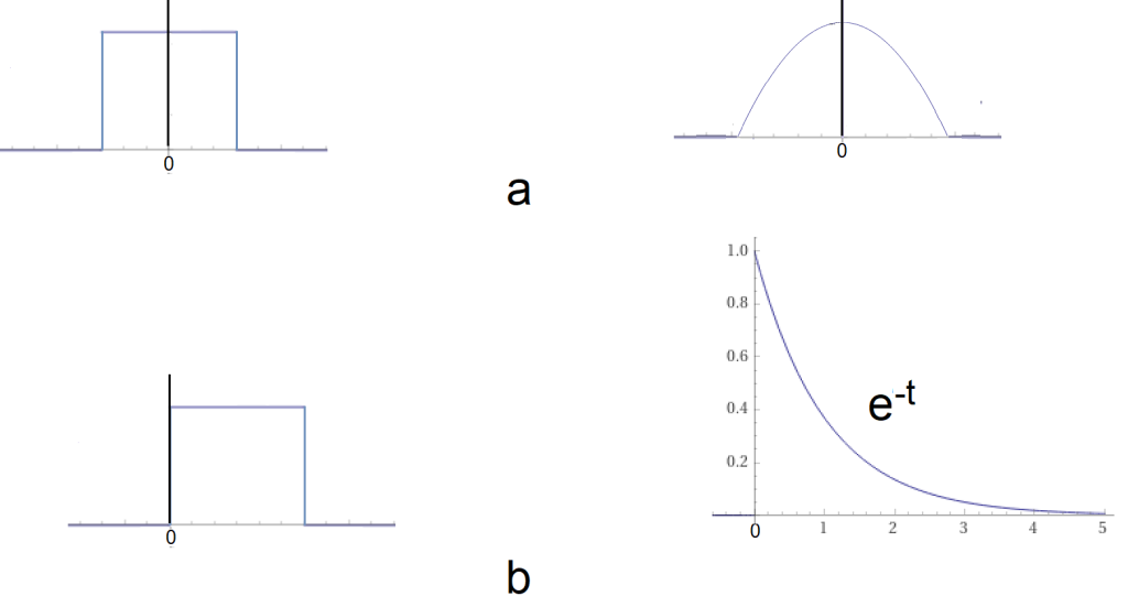
Fig. 5-1
Functions served by the Fourier Transform
They have a finite duration or infinite but with a finite energy/field.
Fig. 5-1a
Even functions
E.g. single pulse A=1, Tp=1sec from chapter 3 and 4. Or a piece of a symmetrical parabola.
Their transforms are “easier” real functions than complex  functions.
Fig. 5-1b
Not necessarily even.
Usually their transforms are more difficult complex functions, and that’s what this chapter is about. The right example, i.e. f(x)=exp(-t) for t=0…+∞ has infinite duration but finite energy/field.  Under certain assumptions, there are even Fourier Transforms  such functions as e.g. f(t)=1 ,t^n, sin(ωt), cos(ωt), dirac impulse δ(t). But not for exp(+x) anymore! On the other hand, almost all f(t) functions are supported by the most general Laplace Transform.
For now, let’s consider a pulse periodic function, that is neither even nor odd..

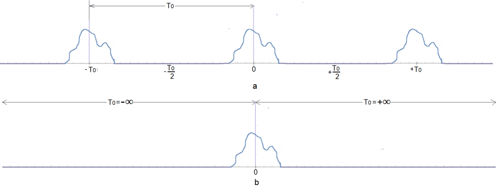
Fig. 5-2a
Periodic function f(t) with period To.
Compared to Fig. 3-1a from Chapter 3, the function f(t) is neither even nor odd.
Fig. 5-2b
The f(t) function is a single pulse in a finite time. We treat it as periodic from Fig. 5-2a with period T=∞.

Chapter 5.2 Trigonometric and Complex Fourier Series
Chapter 5.2.1 What you should know about Fourier Series
Trigonometric and Complex Fourier Series are almost the same in terms of computation. But the latter has some advantages. The complex Fourier coefficients c(n) are the centers of the rotating trajectories F(njω0t)=f(t)*exp(-njω0t) for the Fourier Series in Fig. 5-4a, i.e. for the version with positive and negative ω. Thanks to complex numbers, this is the most intuitive approach to the subject!
Rozdz. 5.2.2 Trigonometric Fourier Series

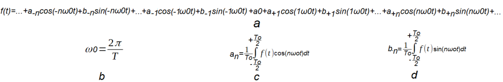
Fig. 5-3
The Trigonometric Fourier Series formula for the function f(t) with period To.
This is a general formula for the function f(t) of the type Fig. 5-2a, which is not necessarily even.
Chapter 5.2.3 Complex Fourier Series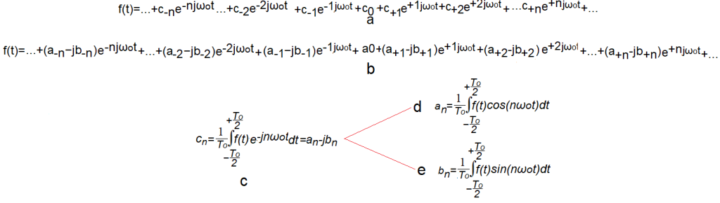
Fig. 5-4
Complex formula for Fourier Series
a. Complex Fourier Series with coefficients c(n)
b. Complex Fourier Series with coefficients as c(n)=a(n)-jb(n)
c. Formula for c(n)
d. Formula for a(n)
e. Formula for b(n)
More about Trigonometric and Complex Fourier Series in the article “Rotating Fourier Series” from the top tab.
Note
The formula c. for c(n) also takes into account c(0), i.e. the constant component. Also applies to Fig. 5-3c..
Chapter 5.2.4 Harmonics Detector
For Fourier Series with positive and negative pulsations ω–>Fig. 5-4a.
The coefficients c(n) are the centroids-centers of gravity scn of the trajectory F(njωt)=f(t)*exp(-njω0t).

Fig. 5-5
Harmonics Detetector for function  f(t)=0.5+0.9*cos(1t)+0.6*sin(1t)+0.6*cos(3t)-0.4*sin(3t)+0.4*cos(5t)+0.2*sin(5t)
The detector searches for harmonics for pulsations ω=-8/sec…0…+8sec. The formula above shows that they are 3 harmonics and the DC component c0=0.5. Each of the above non-zero harmonics corresponds to a pair of oppositely rotating vectors c(n)=c(-n)*. How the detector will detect them? He will start with ω=-8/sec for which he will calculate c(-8)=(0,0). Then it sequentially calculates c(-7) for ω=-7/sec…up to c(+8). Zero c(n)=(0,0) will appear in the center (0,0) of the complex plane. This means no harmonic for this ω. More about c(n) as the centroid of the trajectory, but only for non-negative ω–>chapter 7.7 of the article “Rotating Fourier Series”
In the animation you don’t see the rotating trajectories F(jnω0t), only their effect–>calculated c(n) coefficients as their centroids.
Detector detected below centroids c(n) as complex harmonics amplitudes:
Zero c(n)
c(+8)=c-8)=(0,0)
c(+7)=c(-7)=(0,0)
c(+6)=c(-6)=(0,0)
c(+4)=c(-+4)=(0,0)
c(+2)=c(-2)=(0,0)
Non-zero pairs of conjugates c(n) and c(n)*
These are the amplitudes of complex harmonics for specific ω. Different and not very precise – the harmonics of the function f(t).
c(+1)=0.45-j0.3 i c(-1)=0.45+j0.3
c(+3)=0.3+j0.2 i c(-3)=0.3-j0.2
c(+5)=0.2-j0.1 i c(-5)=0.2+j0.1
DC c(0)
c(0)=a0=+0.5
Check out the animation like:
– ω changes
– for which ω are zero c(n)
– for which ω are non-zero c(n) as pairs of conjugate numbers.
These rotating trajectories and their centers of gravity c(n) serve only to excite the imagination. In fact, the detector computes c(n) according to pattern Fig.5-4c. The animation showed successive c(n), i.e. not very strictly, successive harmonics of the f(t) function.
Chapter 5.2.5 All harmonics together
All c(n) in one picture below. This is a more general equivalent of the bar diagrams from chapter 4 for f(t) which does not have to be even. From the red c(n) vectors, one can read the pulsation ω, the amplitude A and the phase φ of the nth harmonic. The bar diagrams does not show the φ phase. More precisely, it shows but only 0º or 180º.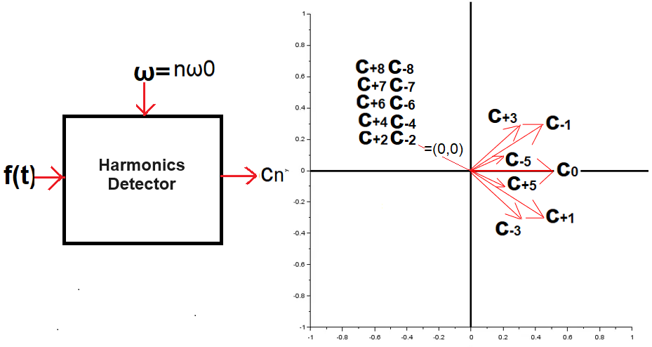


Fig.5-6
All c(n) together
Here it is clearly visible that the zero coefficients c(n)=(0,0), the constant component c(0) and the remaining c(n) as the so-called conjugate numbers.
Now look at the Fourier Series general formula in Fig.5-4a and use your imagination i.e.
– vector c(0) is stationary
– vectors c(+1),c(+3),c(+5) rotate “counter-clockwise” because their c(n)*exp(+jnω0t)
– conjugate vectors c(-1),c(-3),c(-5) rotate “clockwise” because this is their c(-n)*exp(-jnω0t)
The sum of all of them will give us a vector f(t) moving along the real axis Re z.
Conclusion
The rotating vectors should be a Fourier Series for you in Fig.5-4a.
Note
1. Animation of oppositely rotating vectors for another f(t)–>Fig.12-8 in chapter 12 of the article “Rotating Fourier Series” from the tab from above.
2. This data can be directly accessed from the function f(t), where the DC component and harmonics are visible. But our detector calculated them “not seeing” the individual harmonics, only their sum! As if it only used the f(t) graph.
3. Many authors boast that they don’t use complex numbers to explain things. That it will be easier. But complex numbers make it very easy to understand Fourier Series! The integrand of f(t)exp(-jω0t) is a rotating trajectory around the point/vector c(n)=a(n)-jb(n). Point c(n) is like the center of gravity of this trajectory, other words centroid. It is also the complex amplitude of the harmonic a(n)*(nω0t)+b(n)*sin(nω0t)=|cn|*cos(nω0t-φ). This can be clearly seen in the animation  “Rotating Fourier Series” –>chapter. 12-->Fig.7-7.
4. The topic was discussed in “Fourier’s Rotating Series” chapter 7.5 , but only for non-negative pulsations–>ω=0…+7/sec,+8/sec. The coefficients c(n) had twice the amplitude and, of course, there were no conjugate coefficients c(n)*. In the complex plane on the real axis, the vector moves according to function f(t). So swings around the point (0,0). This plane will begin to rotate with velocities ω=-8/sec,-7/sec…0…+7/sec,+8/sec. The function f(t) draws trajectories F(jnω0t)=f(t)*exp(-njω0t) for n=-8…0…+8 and ω0=1/sec. That is, with velocities ω as above. At each speed ω, the trajectory will of course have a different shape and a different center of gravity scn equal to the coefficient c(n) in Fig. 5-4c. When f(t) has no harmonic for ω, e.g. for ω=+2/sec, then c(n)=0.