31. Influence of Non-linearity on Control - How does it work?/Jak to dziala?

Automatics

Chapter 31 Influence of Non-linearity on Control
Chapter 31.1 Introduction
The most influential non-linearity on the control process is saturation in the power amplifier (another name – actuator) in front of the controller. Therefore, the title of the chapter could be more explicit – “Impact of actuator saturation on the quality of control”. You’ll soon know what it’s all about. Even one non-linear element “spoils” the whole scheme. So you can’t uncritically apply the theory you’ve learned so far, in which all elements were linear.
Transmittance reminder.
When you use transmittance it means you are in linear objects. In these objects, the output signal y(t) in steady state is proportional to the input signal y(t).

Fig. 31-1
Characteristics of a linear object in a steady state.
And in the unsteady (or transient) state, linear objects are governed by linear differential equations, in which all coefficients at y(t), y'(t), y”(t), … x(t), x'(t), … are constant. such as:

Fig. 31-2
Differential equation of a linear object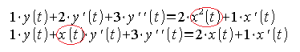

Fig. 31-3
Examples of differential equations that are not linear
The red ones are bugs that make the differential equation not linear, read – difficult to solve. Let’s return to the linear differential equation in Fig. 31-2, which corresponds to the transmittance G(s).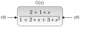

Fig. 31-4
The transmittance G(s) which is described by the differential equation in Fig. 31-2
For the exercise, associate parameters 1, 2 and 3 of the numerator and 1, 2 of the denominator of the above transmittance G(s) with the linear differential equation in Fig. 31-2. If you have problems, look at Fig. 15-7 in chapter 15. So far, we have dealt with linear objects all the time, except for the chapter on on-off control. And only for them the concept of transmittance G(s) makes sense. G(s) transmittances correspond to linear differential equations, and these have long been figured out by mathematicians. Therefore, the theory of the behavior of linear dynamic objects is very elegant. From the transmittance G(s), it is relatively easy to predict how the system will behave after closing it with a feedback loop. Will it be stable? What will be the steady state? How to select the parameters of the PID controller? If at least 1 non-linear element appears in the block diagram, then (almost 100%) the entire object will become non-linear. That is, one that can no longer be described by a linear differential equation.

Chapter 31.2 Non-linear elements
Chapter 31.2.1 Introduction
Examples of non-linear elements.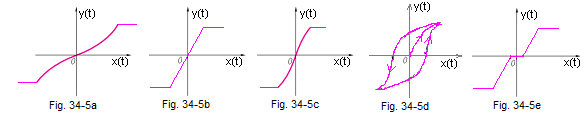

Fig. 31-5
A typical feature of each real object (and not an ideal one!) is that sooner or later it reaches a state of saturation. For example, for an amplifier, saturations are +/-15V supply voltages. This can be seen in the characteristics above. Well, maybe apart from Fig. 34-5d.
Typical non-linear characteristics
Fig. 31-5a – “increasingly faster with saturation” – A strange but accurate name.
Fig. 31-5b – linear with saturation
Fig. 31-5c – “increasingly slower with saturation”.
Fig. 31-5d – hysteresis. Note that the value of y(t) depends on whether x(t) is increasing or decreasing. Here you can’t see +/- saturation. They would appear with larger amplitudes of the input signal x(t).
Fig. 31-5e – linear with dead zone and saturation
In the next 2 subsections for element inputs:
-linear with saturation (b)
-linear with dead zone and saturation (e)
we will give the black sine wave x(t) and examine the red response y(t).

Chapter 31.2.2 Non-linear element with saturation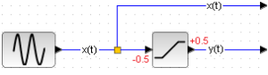

Fig. 31-6
Non-linear element with saturation and sine input x(t)

Fig. 31-7
Saturation occurs at y(t)=+/-0.5.
Before saturation x(t)=y(t)
After saturation
for x(t)>0.5 y(t)=+0.5
for x(t)<0.5 y(t)=-0.5
If the saturation was +/-1, it would be x(t)=y(t) all the time and you would see red sine wave y(t).
Chap. 31.2.3 Non-linear element with dead zone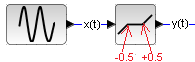

Fig. 31-8
Non-linear element with dead zone for sinusoidal x(t)

Fig. 31-9
The dead zone exists for -0.5….+0.5.
If the dead zone was zero (otherwise-it doesn’t exist), then it would be x(t)=y(t) all the time and you would see a red sine y(t).
If the dead zone was in the range -1…+<1, it would still be y(t)=0 and you would see a flat red y(t)=0 and a black sine x(t).

Chapter 31.3 How does an ideal control system work?
A typical control system with a PID controller and a two-inertial object. You have already met him in Fig. 27-18 chapter 27. It can be, for example, a temperature controller with a 1 kW heater output. The heater is immersed in a small tank with liquid. Let’s assume that the liquid is perfect, i.e. it neither freezes nor evaporates. We expect that in the steady state there will be zero error e(t), i.e. y(t)=x(t)=+1.

Fig. 31-10
Let +1 be +100°C.
And we rightly expect e=0, because there is an integral component I. The output temperature reached +100°C after only 1.5 seconds! Then there was a slight overshoot of +10 °C and after 10 seconds a steady state y(t)=x(t)=+100°C occurred. On the other hand, the sPID(t) control signal has large overshoots. “Positive” power – heating is sometimes greater than +2, “negative” power – cooling lower than -1. Therefore, the temperature y(t) reached the steady state very quickly, after only 1.5 seconds, although the object has 2 inertias of 3 seconds and 5 seconds!
This is the good job of negative feedback, more generally – automatics. If it was an open system, read without feedback, it would take half a minute, not just 1.5 seconds. You are also using negative feedback by yourself when cooking soup. You turn the gas up to full and then turn it down when the temperature reaches the boiling point. I talked a bit, so let’s go back to the time charts. The sPID(t) control signal is clearly visible, cut off by the oscilloscope at the level -1 and +2, i.e. -100°C … +200°C. To see how large these overshoots of the sPID(t) control signal are, let’s change the range of the oscilloscope from -1…+2 to -20…+160. So at -2000°C…+16000°C! I remind you that in our course there are liquid temperatures lower than -2000 ° C and higher than +16000°C.

Fig. 31-11
Although the signals x(t), y(t) of approx. +100°C are barely visible now, you can see the whole sPID(t) control signal . At the beginning, the sPID(t) varies between -5…+160. So for a short moment the positive (heating) power “wants” to heat the liquid to +16000°C and in a moment the negative (cooling) power “wants” to cool down to -500°C! In the steady state, the control heater draws 1kW, but during the peak, as much as 160kW! After all, no constructor will give such a huge heater! Maximum 3 kW. Negative power-cooling is also rarely used. Therefore, the narrower range 0…3 instead of -5…+160 will be the limitation. Even narrower. After all, when the power is turned off, the temperature drops not to 0°C, but to the ambient temperature, e.g. +20°C. This is where theory differs from practice*. The linear systems we have considered so far are elegant, easy (relatively, relatively!) and answers many general questions. Stability, Hurwitz, etc. On the other hand, real systems – non-linear will differ from linear ones.
How far to deviate? How much worse they are? How reliable is their linear approximation? This will be discussed in a moment.
* Once in a noble automatic company I saw a poster with its motto:
– Practitioner – Everything works, but doesn’t know why.
– Theorist – Nothing works, but he knows why.
We combine theory with practice. Nothing works and we don’t know why.
I liked them right away.

Chapter 31.4 How does a real automation system work?
Chapter 31.4.1 Introduction
There are no ideals in life. The transmittance G(s) is only an approximation of the real object. The question arises. How far is it from reality. The first approximation of a real system is something like this.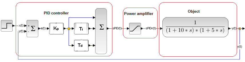

Fig. 31-12
In the following points I will try to justify that the non-linearity is mainly introduced by the Power Amplifier. Therefore, we will consider the Power Amplifier, PID Controller and Object in this respect
Chapter 31.4.2 Power Amplifier with Saturation
The diagram differs from Fig. 31-10 only with the Power Amplifier in the middle of the diagram. So far, we have assumed that the signal from the sPID(t) controller always has sufficient power to control the object. It is known that this is not so. Each amplifier has its own saturation. Even the big power plant i will not generate more than 4,000 MW. It is also a gigantic power amplifier. The input is the power knob (it doesn’t matter if it’s computerized) in the Central Dispatch Room, and the output is the power given to the energy network.
The Power Amplifier in the diagram is nothing but a linear element with saturation from Fig. 31-5b. It does not have to be in the electric version. It can be, for example, a valve with an actuator. The signal from the controller controls the degree of valve opening, thus indirectly the flow, e.g. the supply of steam to the turbine. The flow F will not be arbitrary, only in the range of 0 … Fmax So again we have a Power Amplifier. The electric power amplifier or valve or something else is collectively called the actuator. All right, we have the actuator, which as a non-linear element spoils the whole scheme. It spoils, i.e. the transmittance of the entire opened and closed system cannot be calculated. What about PID and object?
Chapter 31.4.3 PID controller
This is an almost perfect linear system with transmittance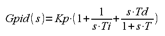

Fig. 31-13
The controller settings can be e.g. as follows:
Kp=10
Ti=7 sec
Td=2 sec (derivative, as in any decent controller, is real, i.e. with T inertia)
One more comment on “almost perfect linear system”.
Modern PID controllers are usually implemented in microprocessor technology. So the response of the controller is not continuous but quantized by the clock pulses. However, with frequent quantization, the controller response can be treated as continuous. The output of the controller is a digital/analog converter. So a continuous signal enters the power amplifier. By assumption, the power amplifier will enter saturation earlier than the PID. Therefore, with a clear conscience, we can treat PID as the transmittance Gpid(s).
Chapter 31.4.4 Object G(s)
The object can be a furnace, a rectification column or a rocket. Of course, each of them has different dynamic properties. In Fig. 31-12, an example object is a two-inertial unit. So we assumed that it is a linear unit with transmittance G(s).
There are weaker linearity arguments for the object than for the PID. The static characteristic of most typical objects is “increasingly slower with saturation” –>Fig. 31-5c.
What is the conclusion? The fact that the denominator, i.e. the slope of the characteristic, is equal to unity for the zero operating point. and then it decreases. Similarly, the time constants can vary within certain limits. So the “true” transmittance parameters may depend on the operating point and the true value is kind of fuzzy within the limits.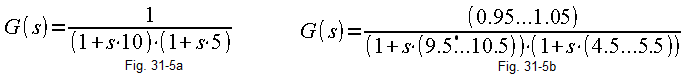

Fig. 31-14
Fig. 31-15a-based on the observation of the object, or on the basis of the mathematical model of the object, we assume that it is a two-inertial object with gain k=1, time constants T1=10 sec and T2=5 sec.
Fig. 31-15b-The true parameters can be, depending on the operating point and measurement error, in the ranges k=0.95…1.05, T1=9.5…10.5 sec and T2 4.5…5.5 sec.
Many objects, especially multi-inertial ones, can be approximated as inertia with delay. Why? An exact model is better than an approximate one. It’s better to be healthy and rich than poor and sick.
First, it is easier to determine its parameters K, T and To by observing the response to a unit step.
Secondly, for the transmittance determined in this way, the parameters of the PID controller settings are already ready. Then the response of the PID-controlled system is optimal under some criterion. For example, the shortest control time with possibly small overshoots.
The T inertia with To delay and K gain have already been mentioned much earlier. As a reminder, I will show the response of y(t) to the x(t) unit step.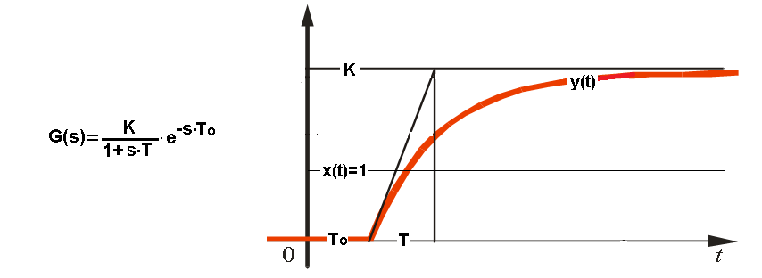

Fig. 31-15
Inertia with delay.
Chapter 31.4.5 Conclusions
Referring to Fig. 31-12, we found that:
– The PID controller is a linear object with transmittance Gpid(s)–>Fig. 31-13
– With some forbearance, the object G(s) is also a linear object. The closer to linearity the smaller the input signal.
Often objects are approximated by inertia with a delay.
– The actuator is a linear element with saturation, i.e. it is a non-linear element. Mainly, it “spoils” the whole system, depriving it of linearity. So it is impossible to calculate the transmittance from Fig. 31-12.
– All the theory taught so far –> stability studies, selection of controller settings, etc…, concerns linear systems.
Considering that in real control systems there is always an actuator, we can conclude that the whole control theory is just a beautiful mathematical trinket. There are no material benefits in it, only spiritual ones. Fortunately, it’s not quite like that.

Chap. 31.5 Comparison of an ideal and a real system
Chap. 31.5.1 Introduction
We will study the response to x(t)=+1 unit step, and z(t)= +0.4 and z(t)=-0.4 disturbances at actuator saturations of 0…+1.5 and 0…+5. Common sense expects that the later saturation occurs, the more ideal the system is. Also, reducing the x(t) step amplitude has the same effect. What about the z(t) disturbance? It will turn out that the responses to a small disturbance are similar for real and ideal systems. The more the less disturbance.
In the next experiments, the PID controller with the settings Kp=10, Ti=7 sec, Td=1.5 sec will control a two-inertial object with the parameters K=1, T1=10 sec and T2=5 sec. as optimal for this object. Assuming, of course, that the object was ideal linear.
Chap. 31.5.2 Saturation 0…+1.5, x(t)=+1, z(t)=+0.4 (heating)
We have 2 identical tanks with identical liquid next to each other. The parameters of the controllers are also identical. The difference is only in the power of the heaters.
The first-ideal system has an unlimited power. So there are no saturation. It can even give a heating power of +1 000 000kW and a cooling power of -1 000 000kW when needed.
The second real-system already has a real actuator, i.e. a heater with a limited power of +1.5 kW. In addition, a negative signal from the controller does not cool, but turns off the heater. The temperature then drops to the environment, e.g. to 0°C. So the controller range is 0…+1.5 kW.
The disturbance is the activation of the +0.4 kW heater. x(t) setpoint and z(t)+0.4 disturbance act in parallel on 2 systems. For sure Ideal will be better than Real. But how much better? Will it be 100:0 or just only 5:2 as in football match score?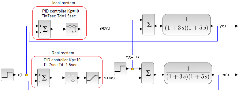

Fig. 31-16
At the top there is an ideal system, i.e. with an actuator without saturation.
At the bottom there is a real system with an actuator with saturation 0…+1.5.
How to interpret it? The maximum value of the controller corresponds to the heater power of +1.5 kW, which in a steady state will give a liquid temperature of +150°C. Lower saturation 0 kW means the heater is turned off and the temperature then drops to the ambient temperature, e.g. to 0ºC.

Fig. 31-17
Up to 60 sec, we only have x(t)=1, in 60 sec, there will be a disturbance +0.4-heating.
IDEAL SYSTEM – actuator without saturation
The output signal yi(t) and the control signal sPIDi(t) relatively quickly led to the state yi(t)=1, in which the fixed error is zero. Very large fluctuations of the sPID(t) control signal at the beginning of the x(t) step –>Fig. 31-11. In 60 seconds we have a disturbance z(t)=+0.4–> activation of an additional heater with a power of 0.4 kW. The PID controller correctly assessed the situation and also reduced the power by 0.4 kW. There was, of course, a transitional state of several seconds, but everything ended as it should.
REAL SYSTEM actuator with saturation
Previously, the control signal sPIDi(t) could roam within the limits of -infinity …+infinity, now the actuator gives only a modest sPIDr(t) within 0…+1.5. Therefore, instead of the 160 pin, there is a green flat time chart with an amplitude of +1.5 from the beginning of the step to about 18 sec.
Good and that. During this time, yr(t) tends to +1.5 instead of 160. Therefore, yr(t) increases more slowly. In addition, there is a large overshoot to approx. +1.3, because the braking from the derivative element D is weaker than in the ideal case. Note that then the green control signal sPIDr(t) no longer enters saturation and therefore yr(t) comes to 1 in steady state (zero error), as in any decent linear system, i.e. ideal. Despite the fact that overshoot and control time are greater in the real system, they are not 100 times greater, as if they resulted from the maximum signals sPIDi(t)=+160 and sPIDr(t)=+1.5.
In the 60th second, a disturbance z(t)=+0.4 occurred. The yr(t) and yi(t) time charts now perfectly coincide because no saturation worked. The real system now thinks it’s ideal.
Conclusion
Non-linearity, including mainly the saturation of the actuator, obviously deteriorates the quality of control, but not so much!

A note that you may not read, because there has already been something about it
What do Kp, Ti, Td do?
Kp=10-proportional
It quickly brings the output signal yi(t) to 0.91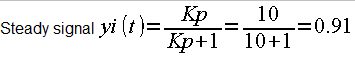

Fig. 31-18
So the Kp component does not ensure zero control error.
Ti=7sec-integrating component
Brings the error to zero. Question. If the integrating component brings the error to zero, then what the hell is Kp for? The answer is simple. Kp quickly brings yi(t) to 0.91. The I component also reduces the error to zero from the very beginning, but it does so slowly. In short and not very precisely – Kp quickly makes yi(t)=0.91, and Ti is responsible for the rest, i.e. for bringing yi(t) to 1.
Td=1.5 sec-differetiating component
Even more than Kp, it speeds up the approach to yi(t)=1. At the very beginning of the step, Kp gives a kick in the sPID(t) signal to the value of 10, and for the rest, i.e. 150, corresponds to the differentiating component, i.e. Td. After all, this differentiates the x(t) step. And so it is fortunate that this is real and not ideal differentiation. Then we’d have an infinitely large pin, not a miserable sPID(t)=160.
Let’s go back to that x(t) kick. Thanks to it, yi(t) grows very quickly. As if he wanted to go not to 1 but to 160. In a moment x(t) is flat–> sPID drops quickly. But differentiation from increasing yi(t) works. And it works in the opposite direction of the initial 160 kick! It even gives negative sPID(t) values for a while. And what does that mean? That the Td component now acts as a brake or stabilizer. This prevents overshoots and even instability
Chapter 31.5.3 Saturation 0…+1.5, x(t)=+1, z(t)=-0.4 (cooling)
The diagram differs from Fig.31-16 only in the disturbance. Previously it was z(t)=+0.4-heating, now it’s z(t)=-0.4-cooling

Fig. 31-19
The time charts up to 60 sec are identical to Fig. 34-18. To the disturbance z(t)=-0.4-cooling, the controller reacted correctly by increasing the heating power by +0.4. The control signal has not entered saturation, the controller “thinks” that the system is linear. Therefore, the sPIDi(t) and sPIDr(t) signals coincide.
Chapter 31.5.4 Saturation 0…+5, x(t)=+1, z(t)=+0.4 (heating)
This and the next scheme differ from the previous ones only in saturation. It will now be greater 0…+5 instead of 0…+1.5. Bigger, i.e. the system is more “ideal”, i.e. we expect better control. We now have a more powerful actuator->read more expensive.

Fig. 31-20
In Fig. 31-17, you saw the effect of saturation +1.5 on the real control signal sPIDr(t)– (after the power amplifier). There is a higher upper saturation here – +5, and that’s why you can’t see this green and flat sPIDr(t). In any case, the higher maximum sPIDr(t) resulted in faster control and less overshoot. It can be said that the system has come close to ideal. The response to a disturbance has not improved, because it is still the same as for an ideal system. Why? Because the sPIDr(t) control signal did not enter saturation.
Chapter 31.5.5 Saturation 0…+5, x(t)=+1, z(t)=-0.4 (cooling)
The scheme differs from the previous one only in the disturbance z(t)=-0.4 (cooling).

Fig. 31-21
The difference is only in the reaction to the disturbance z(t)=-0.4-cooling.
Chap. 31.5.6 Conclusions
Compared to the Ideal system, the Real system comes to a steady state more slowly and with greater overshoots. This is of course a downside, but you can live with it. Especially that zero error is ensured and disturbance suppression is almost identical to the ideal one. Also take into account that the automatics mainly suppresses disturbances z(t) and changes of the setpoint x(t) are much less frequent. Although the ideal system gives more than 100 times more kick than the real system at the beginning of the step (160 to 1.5), the reaction is not 100 times worse – read slower. Therefore (with some leniency) we can treat real systems as linear. But only when x(t) is between the saturation of the actuator–> in our case x(t)=0…+1.5.
This condition is not difficult to meet. And this means that for real systems we can use all the rich knowledge for linear systems.
Coming back to football, the relationship between the Ideal and the Real system is more Germany-Austria than Germany-Gibraltar.

Chap. 31.6 How does the system behave when the setpoint x(t) is greater than saturation?
Chap. 31.6.1 First attempt – only x(t), yi(t) and yr(t)
The maximum power behind the controller is +0.95 kW, which is able to heat the liquid to +95°C. But I want the controller to heat the liquid to +105 °C. It is physically impossible! As if the manager demanded from the employee to perform a task above his competence.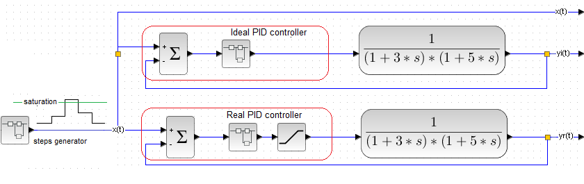

Fig. 31-22
This time it will not be a single unit step of the setpoint x(t), but a signal from the step generator. The real PID controller has limits 0…+0.95 on the output of the actuator.
There will be 3 periods for step x(t) where:
Period 1
x(t)=+0.3 (below saturation)
Period 2
x(t)=1.05 (above saturation!)
Period 3
x(t)=+0.5 (again below saturation)
The reactions of ideal yi(t), i.e. without saturation, are obvious. Negative feedback will work, which will bring the zero error. The signal yi(t) tries to imitate x(t). The entire course so far has tried to convince you of this. And the reactions of the controller with saturation, i.e. real? Try to anticipate them. For now, we are not interested in the “internal” signals sPID(t), sPIDir(t) and sPIDr(t) from Fig. 31-22.

Fig. 31-23
The performance of the ideal yi(t) controller is always better than the real yr(t). Therefore, let us examine only the real yr(t).
Period 1. x(t)=+0.3
Setpoint x(t) is less than saturation=+0.95. So there will be feedback. The signal yr(t) will go to x(t)=yr(t)=+0.3.
Period 2. x(t)=+1.05
The setpoint x(t) makes the real controller reach the state yr(t)=+1.05, i.e. the output temperature +105°C. But how is the poor PID supposed to do that when the actuator has a saturation of +0.95? It’s not possible! Simply yr(t) will tend to +0.95. Negative feedback won’t work! As if it was an open system.
This can be seen in the time chart, where only at the end of period 2 the signal yr(t) reached a steady state of +0.95.
Period 3. x(t)=+0.5
Setpoint x(t) is less than saturation=+0.95. So a negative feedback will work which will bring the error to zero–>yr(t)=x(t)=+0.5. Of course, the real yr(t) is slower (worse!) than the ideal yi(t). But where did the extra dead time come from that wasn’t there in period 1? After all, this phenomenon did not exist then. Dead time is extra delay The one that is always bad for control!
Chapter. 31.6.2 Second attempt – more accurate
To the previous diagram, we will add the observation of the control signal of the ideal yellow sPIDi(t) and the actual black sPIDr(t) from Fig. 31-22. Maybe we’ll learn something about dead time?

Fig. 31-24
The signals of an ideal system are obvious. The stronger and shorter sPIDi(t) resulted in the usual fast response of yi(t) which clearly tries to mimic the stepped x(t) in periods 1, 2, and 3.
Let us then consider a system with a real controller, i.e. with saturation.
In period 1, the regulator did not reach saturation. Therefore, negative feedback kicked in and the signal yr(t) tried to track the stepped x(t). However, it did it worse (longer!) than the ideal one, although in steady states it also gave zero error –>x(t)=yr(t)–>e(t)=0! Also note that in steady state, the actual control signal is sPIDr(t)=yr(t). As in ideal sPIDi(t)=yi(t).
In period 3, it’s similar, but dead time appeared out of nowhere. The most important thing is that the feedback worked and yr(t) reached x(t)=+0.5.
In period 2, the regulation entered saturation. I.e. x(t)=1.05 is greater than saturation=0.95 of the maximum signal of the actual controller, i.e. sPIDr=0.95. This means that negative feedback does not work and yr(t) reaches a steady state of yr = 0.95, as in an open system..

Chapter 31.6.3 Third approach – even more thorough
We observe yellow ideal sPIDi(t), black real sPIDr(t) and green sPIDir(t) in front of the actuator in Fig.31-22

Fig. 31-25
Ideal system
The time chart of the yellow sPIDi(t) is obvious and requires no comment.
Real System
The green sPIDir(t) signal in front of the actuator can have any numeric value because it is calculated by the microprocessor and does not contain power. The letter i in sPIDir(t) suggests that the signal is after the ideal part of the real PID controller.
Period 1 x(t)=+0.3
Until tz=6.5 sec the green sPIDir(t) is greater than +0.95 saturation. This will result in cutting of the the black sPIDr(t). Then yr(t) tends to +0.95 as in an open system. Feedback will occur after tz=6.5 sec when sPIDi(t) drops below +0.95. Then it will reduce the output signal yr(t) to yr(t)=x(t)=0.3. Fast but of course slower than yi(t) in the Ideal System.
Period 2 x(t)=+0.95
Green sPIDir(t) jumped up. And what happens to it next, is not visible because the scope of the oscilloscope is too small. Anyway, the signal after the actuator is cutted at sPIDr(t)=+0.95 and yr(t) tends to +0.95 as in open circuit (no feedback). You can’t see all the green sPIDir(t)! And interesting things happen there. You will find out in the next experiment.
Period-3 x(t)=+0.5
I guess there’s something dawning with dead time. It can be seen that at this time yir(t) is greater than +0.95. Then yr(t) is roughly truncated at +0.95 as well. When yir(t) becomes less than +0.95 the feedback will bring yr(t) to +0.5.
Chapter 31.6.4 The same, only a larger oscilloscope range
We will get visually the same scheme, but with a different oscilloscope range -100…+140, previously -1…+2. This will allow you to see what was not visible in Fig. 31-25.

Fig. 31-26
Signals x(t), yi(t), yr(t) are now tiny, tiny. However, the control signals sPIDi(t) and sPIDir(t) are visible. The green sPIDir(t) mostly covers the yellow sPIDi(t).
Period 1 x(t)=+0.3
Falling green yir(t) pin until tz=6.5 sec. You didn’t see it in Fig. 31-25.
Period 2 x(t)=+0.95
Feedback does not work all the time because sPIDir(t)>0.95. Therefore, we have the classic PID response to a positive unit step in an open system!
Period 3 x(t)=+0.5
The setpoint x(t) has decreased from +1.05 to +0.5. So we have again the classic PID response to a negative unit step x(t). It is now clear that the dead time is the rise of the integral component of the PID controller to a value where sPIDir(t) becomes less than saturation +0.95. Then the feedback will bring yr(t) to yr(t)=x(t)=0.5–> zero control error.
Chapter 34.6.5 Conclusions
1. If the real controller “tells” the object to enter a state that is possible to meet* by the actuator, then the control works in a way similar to an ideal system (with feedback). The response yr(t) is of course slower (worse) than for an ideal one, but in the end yr(t)=x(t) so zero control error will be ensured.
2. If the real controller “tells” the object to enter a state that is impossible to meet, i.e. when x(t)>0.95, then the output signal yr(t) slowly reaches the saturation state as in an open system -> period 2 in Fig. 31-25.
3. If the real controller goes out of saturation, as in period 3 in Fig. 31-25, a dead time will occur. The reason for this is the integral component of the controller->period 3 in Fig.31-26. Another name for the dead time of the PID controller is the integral dead zone.
How to fight the integral dead zone?
Dead time To introduces a delay into the system which is obviously a disadvantage. Because would you like to drive a car in which you turn the steering wheel to the left and the wheels react only after To=1 sec?
Currently, the controller are made in microprocessor technology. Therefore, when the controller finds that despite the control signal increasing from the integral component, the output signal does not increase, it turns off the integral component. So in the saturation state, the PID controller becomes the PD controller.
This is an example of a controller with a variable structure. This switching can occur, for example, when the actuator enters the saturation state, and it is easy to detect by the microprocessor controller.