Complex Numbers

Chapterł 3  Complex functions
Chapter 3.1 Introduction
You can now add, subtract, multiply and divide complex numbers. It’s time for functions.
In electrical engineering, automatics and the like, the complex function is mainly used:
-rational function
-exponential function with base e
Other complex functions, e.g. trigonometric, logarithmic, are used less often and we will not deal with them.
Time charts of complex functions are more complicated than of real functions. To each two-dimensional point in the z-plane we assign a complex number f(z), which is also a two-dimensional. We enter four-dimensional space! Hard to imagine for an ordinary bread eater. We will come back to this topic.

Chapter 3.2 Complex rational functions
We will calculate it using only addition, subtraction, multiplication and division.
We get any power of z by successive multiplications.
Free polynomial z, or “sum of powers” by exponentiation, addition and subtraction
Any rational function, i.e. the quotient of polynomials, by means of exponentiation, addition, subtraction and division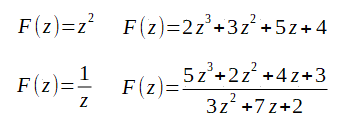

Fig. 3-1
Complex rational functions

Chapter 3.3 Complex exponential function exp(z)
Chapter 3.3.1 Definition
Strictly-exponential with base e, otherwise exponential.

Fig. 3-2
Complex function exp(z) with base e, i.e. an exponential function
Chapter 3.3.2 Number e=2.7182818…
The irrational real number e=2.71828… is the fourth one to know after 0.1 and π. Everyone knows where 0 and 1 came from*. The number π=3.14… is the circumference to the radius. But the number e? Is there any simple “circumference to radius” interpretation for it. It is, but less obvious, and it came from the banking world
*Where exactly is it from?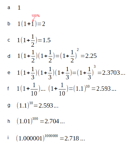

Fig. 3-3
Number e and interest in the bank.
a I put a 1 $ in the bank with 100% interest after a year. By the way, good interest and the bank is great.
b After a year, it should be $2. Note that 1 is 100%
c I made an agreement with the bank that the interest will also be 100% but I will collect money $ 1.5 after six months. Using banking vocabulary – capitalization after half a year
d If I collected it after a year, i.e. after 2 capitalizations, it would be 2.25 $
e And if there were 3 capitalizations, after the 3 year $ 2.3703 …
f $2,593… after after 10 capitalizations
g The same, just a different notation
h PLN 2,704… after a year after 100 capitalizations
j PLN $2,718…. after a year after 1,000,000 capitalizations
The more capitalizations in a year, the closer we are to the so-called continuous capitalization. Then, after a year, 1$ will become $e =2.7182818…
You can easily check the calculations with a calculator.
Note:
The number e is a continuous capitalization of 1 $ 1 after 1 year with 100% interest.

Chapter 3.3.3 The real exponential function exp(x)
Before we get to the complex function version, let’s take a look at the real version. So an exponential function with base e. We can easily calculate it by multiplying the values ​​of these functions for the integer exponent 0, 1, 2, 3...

Fig. 3-4
Exponential function values ​​for integer values
But how to calculate it for e.g. for x=1.234?
We’ll do what all calculators do. i.e. we decompose the function into a power series, e.g. a Maclaurin series.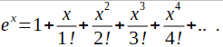

Fig. 3-5
The exponential function as a power series
In this way, we will calculate the value of the function for any x using only 4 basic mathematical operations.
Note:
symbol ! is the so-called factorial
E.g. 3!=1*2*3=6

Chapter 3.3.4 Complex exponential function exp(z)
We can now calculate the value of the exponential function exp(x) for any real x. Let’s do the same thing, but for any complex number z. I wonder how this thing will behave? Maybe it bites, maybe it kicks?
So let’s decompose exp(z) into a complex Maclaurin power series.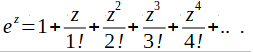

Fig. 3-6
The complex exponential function as a complex Maclaurin power function.

Chapter 3.3.5 The special case of exp(z) or exp(jωt)
Fig. 3-6 can be a definition of a complex exponential function! We can easily calculate its value for any of them using only 4 basic operations that we already know. No problem, but quite tedious because z is a pair of numbers! Also the plot of exp(z) is hard to visualize–>see Chapter 3.1. Therefore, we will consider its special case when z=jωt for t=0…∞ That is, when the domain is the upper half of the imaginary axis Im z. We will therefore consider the complex function exp(jωt), which, as it turns out later, is ideal for analysis sine waveforms. And this is the basis of such fields as electrical engineering, automatics, radio engineering, acoustics…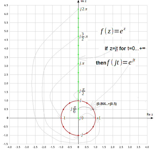

Fig. 3-7
The exponential function exp(z) for z=jt, i.e. for z=jωt when ω=1/sec is the so-called pulsation.
The domain exp(z) is the points 0…∞ of the upper green imaginary semi-axis Im z. The value of the function are the points on the red circle. They were determined by substituting successive numbers into the formula in Fig. 3-6 – green points of the semi-axis Im z. The green points j0, jπ/6, jπ/2, j3π/2 and j2π were marked on it. They are assigned to the appropriate red points exp(jt) on the circle, i.e. +1, (0.866..+j0.5), +j, -1 and -j. There are also other, but not described, intermediate green points on the imaginary semi-axis Im z. Corresponding red points on the circle are also assigned to them.
The formula in Fig. 3-6 shows, for example, that for:
exp(j0)=+1
exp(jπ/6)=0.866..+j0.5
exp(jπ/2)=+j
exp(jπ)=-1
exp(j3π/2)=-j
exp(j2π)=+1
The circle is the graph of exp(jt) for jt=0…∞. But we only examined the range jt=0…2π, ​​for which the image exp(jt) made a full rotation. It will turn out and it can be checked that the second identical rotation will be made for t=2π…4π, the third one for t=4π…6π etc… So exp(jt) is a periodic function!
We were curious how this exp(z) creation would behave? And who would have expected that a complex exponential function could be a periodic function. After all, it bites and kicks!

Chapter 3.3.6 How did the circle in Figure 3-7 come about?
So how did we calculate the values ​​of the complex function exp(jt) for jt=0…∞?
We can’t use Euler’s formula:
exp(jt)=cos(t)+jsin(t)
because we don’t know him yet.
exp(j0)
The first value exp(j0)= exp(0)=+1 is trivial because j0=0 is a real number.
exp(jπ/6)
For jπ/6 it’s not so nice anymore. So we will use the formula Fig. 3-6. There are only 4 basic math operations here, but tiring work. That’s why I recommend everyone a brilliant math tool Wolfram Alfa *
Call up www.wolframalpha.com and do what the drawing says. Just remember that for WolframAlpha, the imaginary number is i, not “electrical” j.
After entering the first 6 components from the Maclaurin series Fig. 3-6 into the dialog box and clicking the appropriate button, the program will calculate the approximation exp(jπ/6).
Note:
Fig. 3-8 is slightly different from what WolframAlfa showed, but the content is the same. I just moved the various elements around to make the drawing more compact. This also applies to subsequent calls to WolframAlpha.
*I wrote more about the WolframAlfa program in the Rotating Fourier Series course in chapter 11.2.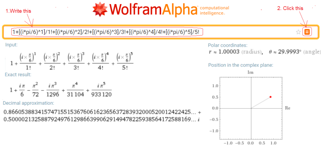

Fig. 3-8
exp(jπ/6) as the first 6 components of the Maclaurin series from Fig. 3-6
Note that the approximate value of exp(jπ/6)≈0.866…+j0.5… was calculated by the program using only the first 6 components of the power series. But he did it quite decently. To the casual observer, the result heals almost exactly on a circle of radius r=1 at an angle of π/6=30°. while the calculated data is r=1.00003 and θ=29.9993° as Polar coordinates. The computed exp(jπ/6) is also shown in the complex plane as position in the complex plane. That Wolfram is nice!
The remaining exp(jt) for jπ/2, j3π/2 and j2π will also be calculated using Wolfram Alfa, but with the specialized complex function exp(z).
How does exp(z) differ from the Maclaurin series in Fig. 3-6?
I think two things:
-More ingredients than 6. How much exactly? I don’t know.
-Assumption that the function is periodic.
So let’s calculate.
exp(jπ/2) calculating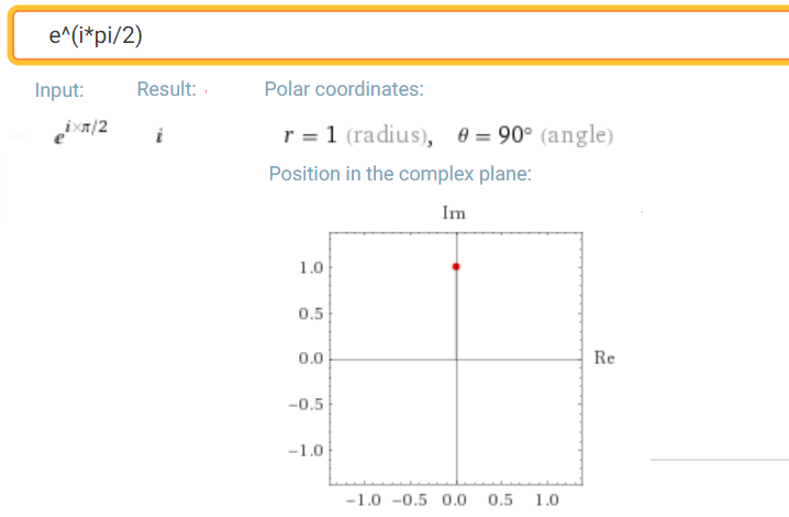
Fig. 3-9
exp(jπ/2)
How perfectly he calculated it!
exp(jπ) calculating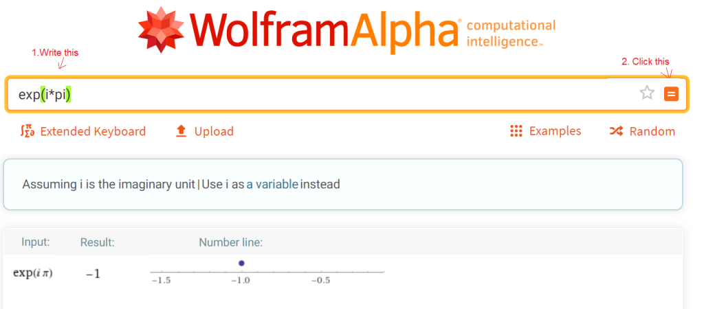
Rys. 3-10
exp(jπ)=-1
Probably
exp(jπ)=-1 or exp(jπ)+1=0
is one of the most beautiful equations of mathematics. In this short formula are used all the most important numbers 0,1,π,e and j.
exp(j3π/2) calculating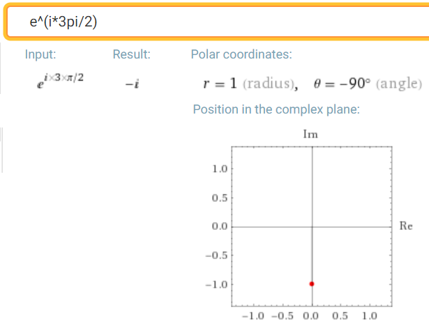

Fig. 3-11
exp(j3π/2)
exp(j2π) calculating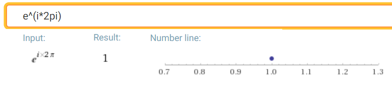
Fig. 3-12
exp(j2π)
Notre that exp(j2π)= exp(j0)=+1

Chapter 3.7 Euler Formula
Returning to the previously mentioned Euler’s formula
exp(jt)=cos(t)+jsin(t)
or more generally
exp(jωt)=cos(ωt)+jsin(ωt)
where ω is the so-called angular velocity in radian/sec, it is more known in the “angular version” where instead of ωt there is angle α.
exp(jα)=cos(α)+jsin(jα)
The formula has been known since the 18th century and has a very easy graphic interpretation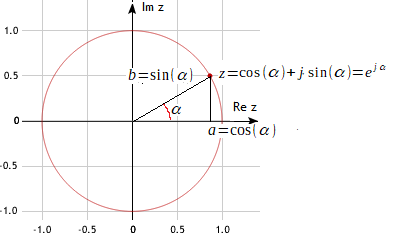

Fig. 3-13
z=exp(jα)=cos(α)+jsin(jα)
Check this formula for e.g. α=0, π/6, π/2, π,3π/2 and 2π and you will get the results you calculated with Wolfram Alfa in Chapter 3.3.5.
E.g. exp(jπ/6)=0.866..+j0.5