Automatics

Chapter 24 PD adjustment
Chapter 24.1 Introduction
The PD controller belongs to the group of PID controllers. Only the integration action has been disabled in it. Unfortunately, it has a basic defect of the P controller. It does not completely eliminate the steady-state error. The closed-loop gain Kz and the steady-state error gain Ke, Ke are also the same as for P-type control:

Fig. 24-1
Go back to the end of the previous chapter and you’ll know why. This means that, for example, for K=100, the steady error is approx. 1%. So what is PD better than P? Improves stability and reduces control time! For the P controller, stability and a small steady-state error are in contradiction with each other. A large Kp provides a small steady-state error, but oscillations and control time increase. The system may even become unstable. Take a look at the typical P-type control.

Chapter 24.2 The ideal differentiating D unit and the real differentiating D unit
Chapter 24.2.1 Introduction
We will examine the response to a step and to a linearly increasing signal. What’s the second for? Because the step gives a Dirac impulse in the differentiator unit, which is difficult to analyze.
Chapter 24.2.2 The ideal differentiating unit response to a  x(t) step

Fig. 24-3
The x(t) unit step  was differentiated. The result is a Dirac hammer response y(t). Let me remind you that the differentiator “calculates” the speed of the signal x(t). And what is the speed of the signal x(t). For t<1sec x(t)=0 and for t>1sec x(t)=1. For these t the signal x(t) is constant. So y(t)=velocity is zero. Therefore, y(t)=0, as you can see in the attached picture.
And what is the velocity y(t) for t=1? Infinitely great! Summa sumarum the output y(t) is a Dirac pulse.
In control, we try to avoid ideal differentiators. They are very sensitive to disturbances, especially to rapid changes, e.g. to electromagnetic disturbances. Rather, the so-called real differentiators are used.
Chap. 24.2.3 Real differentiating unit response to a x(t) step.

Fig. 24-4
An inertial unit with time constant T=0.1 sec was added in series to the ideal differentiating unit. It dampens the unit step before it enters the ideal differentiating unit. We got something similar to a Dirac impulse. Its height is no longer infinite, but has the value y(t)=10. You associate it somehow with the time constant T=0.1sec? I guess so, it’s the inverse of 0.1. A unit step x(t) gives a somewhat strange, hard-to-measure answer. Especially for the ideal differentiating unit. Therefore, a linearly increasing input signal x(t) is better suited for their study. Another name is saw, ramp….
Chap. 24.2.4 Response of an ideal differentiating to a linearly increasing signal

Fig. 24-5
The differentiating unit, as the name suggests, differentiates the x(t) signal to give y(t). For example, for students, the texts in the picture are trivial. For those who have problems with calculus, let it suffice that for the differentiator y(t) is the velocity of black x(t). It is clear that in 5 seconds the signal speed x(t) doubled. Therefore, the y(t) as derivative of x(t) also doubled.
Chap. 24.2.5 Response of a real differentiating to a linearly increasing signal x(t)

Fig. 24-6
That’s what we expected. Where the speed does not change, e.g. after 2 and 6 seconds, it is calculated as a constant of 0.5/sec and 1/sec. However, when it changes (at 1 and 5 seconds), the real unit needs some time to calculate it. This can be a certain, though not decisive, disadvantage. However, the advantage will be resistance to “quick change” type disturbance. They will simply be suppressed by the inertial unit. Next, we will study the PD units, which are a parallel combination of a proportional and a differentiating units (ideal or real). They are not yet controllers, because the input is only a single signal x(t) and not the error e(t)=x(t)-y(t).

Chapter 24.3 The ideal and real PD unit
Introduction 24.3.1
We will also examine the response to a step and a linearly increasing signal.
Chapter 24.3.2 Ideal PD unit response to a step 
Remember!
The PD element is not a controller yet! It does not have a comparator that calculates the error e(t)=x(t)-y(t). Also applies to real controller

Fig. 24-7
At first, the time chart is similar to Fig. 24-3. Only when you look closely will it turn out that there is a proportional component y(t)=1. For the ideal derivative from Fig. 24-3, this component was y(t)=0.
Chapter 24.3.3 Real PD unit response to a step 
How is it different from ideal PD? Compare with Fig. 24-7.

Fig. 24-8
You can see the P component (unit step in 3 seconds) and the real differentiating component (“stretched” peak with a height of 10=11-1).
Chap. 24.3.4 Response of an ideal PD unit to a linearly increasing signal

Fig.24-9
The input x(t) is a linearly increasing signal that doubles the rate of increase in 5 second. In the response y(t) you can see the differential D and the proportional P component. Only in the case when Kp=1, Td=1sec, the P component perfectly coincides with the x(t) excitation. By the way, you see the definitions of the differentiation time Td. This is the time t=1sec for the proportional component P to equal the derivative component D.
Chap. 24.3.5 Response of a real PD unit to a linearly increasing signal

Fig. 24-10
The response is similar to the ideal PD unit. “Smoothing” after 1 and 5 seconds (then there is a change in the speed of the signal x(t)) result from the fact that the real differentiator needs about 0.5 seconds to “recover” and calculate the correct speed. In steady state, the proportional component P and D is clearly visible, which is the same as for the ideal PD unit. I emphasize – the same but only in a steady state.

Chap. 24.4 PD controller with a two-inertial object
Chap. 24.4.1 Introduction
We will study the control system with a two-inertial object, and then in chapter 24.7 with three-inertial. And why don’t we start with a one-inertial one? Because to control this object it is enough to control P from chapter 23.
Here it can be proved, e.g. from the Hurwitz criterion, that for any large gain, even for Kp=1,000,000, the system will always be stable. Not only that, there are no oscillations and the response will be almost a step.
For other objects, adding to a proportional P unit the differentiating D unit  dramatically improves the response. The oscillations may disappear and the system which was unstable with the P-type controller may become stable.
Note
In fact, we will be examining a real and not an ideal PD controller. i.e. in the PD controller, instead of the ideal D, there will be a real differentiating D. It will give a response proportional to the speed of the input signal, which is calculated with some inertia. See Fig. 27-18. This structure will reduce disturbances from high-speed signals that are typical of an ideal D unit.
First, let’s examine the two-inertial object itself. You did this in chapter 23 in p.23.4.2.
Chapter 24.4.2  Two-inertial unit as an open loop

Fig. 24-11
Typical response of a multi-inertial object, here a two-inertial one. We will further explore the PD control with this object at Kp=10 and four different Td=0, 1, 5 and 20 sec. Which Td will give us the best response with as little oscillation as possible and short control time?
Chap. 24.4.3 PD control Kp=10 Td=0 sec
Td=0 means that (real) D differentiation is turned off. So we have a typical P control.

Fig. 24-12
Kp=10 Td=0
So this is the typical P control in Fig.23-9 from the previous chapter. The steady-state gain Kz=y/x=0.91/1=0.91 is consistent with the time chart and theory
Chapter 24.4.4 PD control Kp=10 Td=1 sec
The oscillations in Fig. 24-12 are a bit annoying. So let’s introduce a differentiation component D into the fray. First carefully, a little differentiation. E.g. Td=1 sec. I remind you that all the time we have a real differentiating unit, not an ideal one! Why? I explained earlier. And so it will continue.
What is the difference between the PD controler above and the PD element in e.g. Fig. 24-8? In addition to a different Kp setting, of course. Only that the input is an error e(t)=x(t)-y(t) and not a single x(t). The most important element of the controller appears here, the element that compares the setpoint x(t) with the output signal y(t). It is even more important than the rest of the computational part of the controller – P and D units. Because you can imagine a controller consisting only of a comparator calculating the error e(t)=x(t)-y(t). It is simply a P controller with Kp=1 setting. On the other hand, a controller without a comparison element is meaningless.

Fig. 24-13
Kp=10 Td=1 sec
Didn’t I say that PD improves dynamic properties? Compare only with Fig. 24-12 where there was no D component. The oscillations and control time are radically less. And that was just a little differentiation of Td=1sec. So what will happen when we increase Td to, for example, Td=5 sec? You will learn about it in a moment. As for the static properties, the steady state y(t)=0.91 is the same as for P-control in Fig. 24-12. This is obvious, because in steady state the differentiation of D gives a zero output, i.e. it has no effect on the control.
How to justify better dynamic properties? In other words, a nicer approach of y(t) to the setpoingt 0.91 The easiest way is “Thus says the Queen of Sciences – Mathematics. Exactly, it’s mathematical analysis.
And for the common sense?
1- Steady state is the same as P control in Fig. 24-12.
2-The slew rate y(t) in the first second of the unit  step x(t) is faster, because there is a differentiation of the leading edge x(t), which “boosts” the control signal s(t). In Fig. 24-14, you will examine the same schema, just with different oscilloscope settings, giving you a full s(t) view, not a level 2 cropped view as shown in Fig. 24-14.
It turns out that for t=3 (beginning of the step x(t)) the control signal s(t)=110=100+10!, where 10 is the P component and 100 is the D component. So PD will kick up at the beginning of the step x(t) 11 times larger than the P controller! This should bring it to steady state y(t)=0.91 faster. Not to mention that this kick is 110 times greater than in an open system, i.e. without a controller.
3-Okay, the PD regulator gave a powerful kick up at the beginning of the x(t) step. In this case, we should all the more expect large overshoots greater than ymax=1.2 in the P control in Fig. 24-12. And here it is just the opposite, a tiny overshoot of ymax=1 after 5 seconds.
How to explain it?
It turns out that the component D not only “rushes” the object at the beginning of the  x(t) step, but then “brakes” it. Note that the D component of x(t) that dominates the control signal at the beginning decays to zero quite quickly after some time. This can be seen, for example, in Fig. 24-3. Instead, there is a component D of y(t) acting as a “braking” component. At the beginning, this component is greatest, because the velocity y(t) is the greatest. Then when y(t) settles, it will also disappear. But much later than the D component of x(t)! And the most important. The D component of y(t) is subtracted from the D component of x(t) hence braking. Because that’s how the comparison element works – e(t)=x(t)-y(t). And how does the blue s(t) brake! After all, s(t) sometimes freezes with negative temperature, although the set value is x(t)=+100°C! But thanks to this, the system is very dynamic and quickly comes to a steady state. Differentiation y(t) tries to prevent overshoots. Therefore, the PD control time charts come to a steady state faster and with less oscillation.
PD control was not only created as a result of theoretical considerations of very smart people. The swordsman must hit a specific location of the opponent. It does not have to do it with absolute accuracy, e.g. to the millimeter. It is enough to do it with an accuracy of 5 cm, but quickly! So it is guided not only by the location of the target, but also by the speed of change of the target’s location. He acquires this skill subconsciously through many years of training, gradually optimizing the settings of his private PD controller. Note that zero error, i.e. absolute hit accuracy, is not required here.
I will show again the same time charts  as in Fig. 24-14 with such settings of the oscilloscope so that the entire s(t) control signal  is visible.

Fig. 24-14
It can be seen that s(t)=110! But y(t)=0.91 in steady state, it’s almost on the time axis. The time chart shows us how large s(t) can be. They are exactly the same as in Fig. 24-14, just on a different scale.
Summary
PD at the beginning gives a large control signal s(t) mainly from the differentiation of the x(t) step  so that y(t) comes to a steady state faster. Then it brakes with a differential signal from y(t) in order to reduce the pendulum effect, i.e. to reduce oscillations. The result is a y(t) time chart, that is clearly better than the P control in Fig. 24-12.
What if we could increase the intensity of differentiation even more. E.g. Td=5 sec.
Chapter 24.4.5 PD control Kp=10 Td=5 sec

Fig. 24-15
Kp=10 Td=5 sec
Differentiation is now 5 times more powerful! It would seem that it cannot be better than in Fig. 24-14. And here red y(t) is almost rectangular x(t)! Compare with the red y(t) in Fig. 24-12 of the PD control where Td=0, i.e. P-control. The signal s(t) “cut” by the oscilloscope has the value smax=510 in 3 seconds! So let’s go all the way and let Td=20 sec. Maybe y(t) even better, read-more “rectangular”?
Chapter 24.4.6 PD control Kp=10 Td=20 sec

Fig. 24-16
Kp=10 Td=20 sec
We overdid the differentiation. What too much is not healthy. Not only did oscillations occur, but then the system reaches a steady state y=0.91 only after about 50 seconds. A s(t) in 3 seconds has a value of 2010! This slow approach to the steady state can be explained by too strong “braking effect” of the D signal coming from the y(t) differentiation.
Chapter 24.4.7 PD control Kp=100 Td=0
The settings Kp=10 and D=5 sec in Fig. 24-15 gave us a quick response, with the beginning of one oscillation barely visible. Only the steady signal y(t)=0.91 deviates too much from the setpoint x(t)=1. Indeed, the  error e(t)=1-0.91=0.09 does not bring immortal glory. To reduce it, we increase the gain to Kp=100. So we will study PD control with a two-inertial object with Kp=100 and four different Td = 0, 0.25, 2 and 5 sec. We will start as usual with Td=0, i.e. with P control (without differentiation).

Fig. 24-17
Kp=100 Td=0 means that D differentiation is disabled. So we have a typical P-control. We repeat the experiment in Fig. 23-11 from the previous chapter.
Note
In previous time charts, the control signal s(t) was a blue line. However, this color is quite dominant and often muddied the drawing, a vivid example of which was, for example, Fig. 24-16. Therefore, we will assign yellow to the signal s(t). According to theory, the output signal y(t) reached a fixed value of 0.99 and the steady error e(t) a value of 0.01. However, oscillations and a long time to reach equilibrium are unacceptable. We expect that the D component will help again. As usual, we will start carefully with a small Td=0.25sec.
Chapter 24.4.8 PD control Kp=100 Td=0.25sec.

Fig. 24-18
Kp=100 Td=0.25 sec
It is much faster and less “oscillatory” to reach the steady state y(t)=0.99 (and of course the steady state error e(t)=0.01) than for the P control (because Td=0) in Fig. 24-17. Or can it be better?
Chapter 24.4.9 PD control Kp=100 Td=2sec

Fig. 24-19
Kp=100 Td=2 sec
y(t) itself has a small oscillation. Instead, the control signal s(t) is ho, ho! It is typical that the oscillations of the control signal s(t) are much larger than y(t). Even when y(t) seems to be asleep, s(t) is still making some back and forth movements. The response is better than Td=0.25 sec in Fig. 24-18. So let’s increase Td even more?
Chapter 24.4.10 PD control Kp=100 Td=5sec

Fig. 24-20
Kp=100 Td=5 sec
We overdid the differentiation. The oscillations and control time are greater.
Chap. 24.4.11 Conclusions from the PD control with a two-inertial object
1–The error set for Kp=10 is 0.09% and for Kp=100 it is 0.01% and does not depend on Td. So, as Kp increases, the steady error e(t) decreases. In steady state y(t)=0.99 and e(t)=0.01.
2–For some optimal Td, the D component dramatically shortens the control time and reduces oscillations. For each gain Kp there is an optimal Td for which the response is optimal. That is, with small oscillations (even without) and with a short control time. We found that for Kp=10, Td=5 sec is optimal and for Kp=100 Td=2 sec. There are definitely better settings, because we only did a few experiments.
3–It can be proved, for example, using the Hurwitz or Nyquist criterion, that for any Kp the control with the two-inertial unit is always stable. Another thing is that oscillations with a large amplitude and long duration may then appear.

Chapter 24.5 PD controller with a three-inertial object
Chapter 24.5.1 Introduction
We will do the same as with the two-inertial. We expect more trouble. Indeed, the control time and oscillations will be greater. Moreover, with some gain, the system will become unstable. We will study the control for gain Kp=10 and Kp=25 at different Td. At Kp=25 the error will be smaller, of course, but at certain Td the system will become unstable! This was not in the two-inertial.
We’ll start with a bare object.
Chapter 25.5.2 Three-inertial unit as an open loop

Fig. 24-21
No comment.
Chapter 24.5.3 PD control Kp=10 Td=0 sec
Td=0 means that we have P-type control. So we repeat the experiment from the previous chapter Fig. 23-13.

Fig. 24-22
Kp=10 Td=0, i.e. P control
Time chart with multiple oscillations and long control time. So the P control does not work for this object. The steady-state gain Kz=0.91, or y(t)=0.91 in the steady state, is consistent with the time chart and theory.
Chap. 24.5.4 PD control Kp=10 Td=0.5 sec
We start carefully with a small differentiation Td=0.5 sec.

Fig. 24-23
Kp=10 Td=0.5 sec
Much better than without the derivative in Fig. 24-22. So let’s increase Td by 1.5 sec. Maybe it will be even nicer?
Chap. 24.5.5  PD control Kp=10 Td=1.5 sec

Fig. 24-24
Kp=10 Td=1.5 sec
The time chart is clearly better than Fig. 24-23, and even more so than Fig. 24-22.
Or can it still be improved? E.g. for Td=5sec.
Chapter 24.5.6  PD control Kp=10 Td=5 sec

Rys. 24-25
Kp=10 Td=5 sec
Worse than Td=1.5 sec. Larger amplitude y(t) and more oscillations. It can be assumed that further increase of Td will only make the situation worse.
Conclusions for Kp=10.
It is clearly visible that the object is more difficult to control than the two-inertial one. The optimal differentiation parameter is Td=1.5 sec. The big steady error of 0.09 is a bit annoying. Therefore, let’s try to increase the gain to Kp=25. Probably not for more. I’m afraid of instability.
Chapter 24.5.7  PD control Kp=25 Td=0
I turned off differentiation giving Td=0. So, as usual, we start with the P control.

Fig. 24-26
Kp=25 Td=0
The system has become unstable. Why did I give the formula for the steady gain Kz? Does it make sense when the system is unstable? He has some. Here Kz=0.96 is the constant component of this sine wave y(t). Let’s introduce a small differentiation carefully.–> Td=0.5 sec. Maybe that will stabilize the system?
Chapter 24.5.8  PD control Kp=25 Td=0.5sec

Fig.24-27
Kp=25 Td=0.5 sec
Here you can see the wonderful influence of the differential component D. The system has become stable! Maybe a little too much oscillation. What if you give Td=1sec?
Chapter 24.5.9  PD control Kp=25 Td=1sec

Rys. 24-28
Kp=25 Td=1 sek.
Probably better. Let’s keep looking for luck, maybe Td=5 sec?
Chapter 24.5.10  PD control Kp=25 Td=5sec

Fig. 24-29
Kp=25 Td=5 sek.
We overdid it. Unacceptable.

Chapter 24.6 PD control with disturbances
Chapter 24.6.1 Introduction
The same 2 objects as before will be controlled: two-inertial and three-inertial. Their inputs will be supplied additionally (apart from the setpoint signal x(t) from the PD controller) with the disturbance signal z(t)=+0.5 or z(t)=-0.5. These are powerful disturbances! It is hard to imagine that the network jumps from 230 V to 345 V or to 135 V. I have deliberately provided such a caricature of the network in order to show the main purpose of the control. – disturbances suppression. This is often more important than getting to the setpoint x(t) nicely. If you have a fridge you know why. The temperature setpoint x(t) in your fridge rarely changes (often you have it set at the factory all your life!) and disturbances happen all the time. In the case of disturbances, we chose the settings of Kp and Td determined by us earlier, for which the response to x(t) was optimal. In other words, “the prettiest”.
Note
Note that the response to a setpoint x(t) will be much faster than the response to a disturbance z(t). So the
“closed” transmittance G(s) (“main?”) and the disturbances Gz(s)* are different. This leads to an important conclusion. When designing a system in which you know that the setpoint changes rarely, you should be guided by the optimal disturbances transmittance Gz(s).
*It’s “closed” too but with additional disturbance z(t).
Chapter 24.6.2 Positive disturbance with a two-inertial object z(t)=+0.5 Kp=10 Td=5sec
The disturbance z(t)=+0.5 will appear in 30 seconds.

Fig. 24-30
Up to 30 seconds, i.e. until the appearance of a disturbance, the time chart is the same as in Fig. 24-13 for obvious reasons. The disturbance z(t)=+0.5 caused y(t) to increase to +0.95. So the disturbance was not completely suppressed. Unfortunately, that’s the charachteristic of P or PD control. But without control, i.e. in an open system, the signal y(t) would jump from 1.0 to 1.5!
Note that the setpoint x(t) response is fast and the disturbance response is slow.
Because the disturbance transmittance Gz(s) is different than that of the closed system G(s)!
Note
When the setpoint x(t) changes rarely, select the controller settings  due to the disturbance z(t).
When the setpoint x(t) changes frequently, select the controller settings  due to the disturbance z(t).
Chapter 24.6.3 Negative disturbance with a two-inertial object z(t)=-0.5 Kp=10 Td=5sec

Fig. 24-31
The disturbance z(t)=-0.5 caused a decrease of y(t) to 0.86. Note that the control signal s(t) tries to compensate for the disturbance z(t) by acting in the opposite direction to the disturbance.
This is how any well-designed control system works!
Chapter 24.6.4 Positive disturbance with a two-inertial object z(t)=+0.5 Kp=100 Td=2sec
The disturbance z(t)=+0.5 will appear in 30 seconds.

Fig. 24-32.
The disturbance z(t)=+0.5 resulted in an increase of y(t) to 0.995. There is almost no disturbance effect! It was almost compensated by the decrease in the yellow control signal s(t).
Note
Signals established before  and after the disturbance z(t)
e(t)=0.01 and e(t)=0.005 are close to e(t)=0
and
y(t)=0.99 and y(t)=0.995 are close to x(t)=1
This effect is more visible in Fig. 24-30 when the gain Kp of the controller is lower, i.e. Kp=10.
Chapter 24.6.5 Negative disturbance with a two-inertial object z(t)=-0.5 Kp=100 Td=2sec
The disturbance z(t)=-0.5 will appear in 30 seconds.

Fig. 24-33
The disturbance z(t)=-0.5 resulted in a decrease of y(t) to 0.985. The impact of the disturbance is barely visible. Compare with Fig.24-31 when Kp=10.
Chapter 24.6.6 Positive disturbance with a three-inertial object z(t)=+0.5 Kp=10 Td=1.5sec
The disturbance z(t)=+0.5 will appear in 30 seconds..

Fig. 24-34
Compare with Fig. 24-30. I wanted to write that the system reacts slower to x(t) and z(t), and it turns out that it does. It reacts slower to a jump in the setpoint x(t), but faster to a disturbance z(t)! And yet a three-inertial object is more difficult to control than a two-inertial one! Agreed, but as we already know, the optimal Kp, Td setting for the x(t) be suboptimal for z(t) and vice versa. For a two-inertial object and for Td less than 5 seconds, the response to z(t) will be faster (read – better), while the response to x(t) will be more oscillatory (read – worse).
Chapter 24.6.7 Negative disturbance with a three-inertial object z(t)=-0.5 Kp=10 Td=1.5sec
The disturbance z(t)=-0.5 will appear in 30 seconds..

Fig. 24-35
For a negative disturbance z(t) (e.g. cooling), the controller correctly reacted with an increase in the control signal s(t) (heating).
Chapter 24.6.8 Positive disturbance with a three-inertial object z(t)=+0.5 Kp=25 Td=1sec
The disturbance z(t)=+0.5 will appear in 30 seconds.

Fig. 24-36
The y(t) signal swings a bit. Especially as a response to x(t), because the response to a disturbance z(t) is pretty good. To a positive disturbance (heating), the controller reacted with a decrease in the control signal s(t) (cooling). Thanks to the greater gain Kp=25, the error e(t) in the steady state is smaller than for Kp=10 in Fig. 24-34.
Chapter 24.6.9 Negative disturbance with a three-inertial object z(t)=-0.5 Kp=25 Td=1sec
The disturbance z(t)=+0.5 will appear in 30 seconds.

Fig. 24-37
No comment.

Chap. 24.7 Comparing the PD controller with the P controller
Chap. 24.7.1 Introduction
It’s just like FC Barcelona and and small country football club. We will simultaneously give the same unit step x(t)=1 with disturbance z(t)=+0.5 in 30 seconds. Can you guess which one is Barcelona? We will examine 2 cases with the setting Kp=10 and Kp=100 for a two-inertial object.
Chap. 24.7.2 PD controller Kp=10, D=5 sec and P controller Kp=10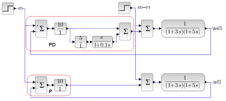

Fig. 24-38
Kp=10 Td=5 sec
Scheme 2 of P and PDcontrols with the same two-inertial object.

Fig. 24-39
PD is unbeatable for the set value x(t) . However, with the disturbance z(t) , the result is debatable, but rather with an indication of PD. But you can always set the PD so that it suppresses disturbances better, at the expense of control for the setpoint x(t). The states established for the PD and P controllers are, of course, the same. In the PD controller, the time to reach a steady state is much shorter (read-better) than for the P regulator.
Chap. 24.7.3 PD controller Kp=100, D=2sec and P controller Kp=100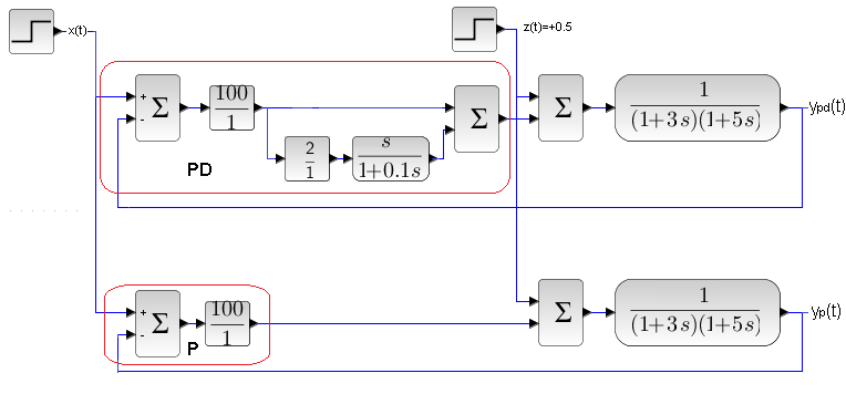

Fig. 24-40
Kp=100 Td=2 sec
Scheme 2 of P and PD control with the same two-inertial object

Fig. 24-41
A crushing advantage of red ypd(t) over green yp(t). That is, PD over P in response to a unit step x(t). Especially since P gives terrible oscillations. As for the suppression of the powerful disturbance z(t)=+0.5 in 30 seconds, for PD and P it is so good at Kp=100 that the influence of the disturbance is almost invisible. So let’s look again at these time charts with a different oscilloscope range of 0.98…1.02. So we’re going to use a loupe.

Fig. 24-42
Here it is clear that the response to a x(t) and z(t) is clearly better for the PD controller.

Chapter 24.8 PD controller with separate differentiation of the output signal y(t)
Chap. 24.8.1 Introduction
The name of the PD controller in the title is quite long. Let it be abbreviated as PDy. Let’s look at the figure below.

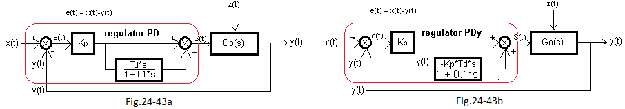
Fig. 24-43
So far, we have used a classic PD controller such as in Fig. 24-43a. The error e(t)=x(t)-y(t) is amplified and differentiated. This is the case in many textbooks and automatics courses. It turns out that when there are slow processes, e.g. in the chemical industry, we more often encounter PDy regulators from Fig. 24-43b. Here only the output signal y(t) is differentiated, not the error e(t).
By the way – I use the term “differentiated” for short, instead of “differentiated with an inertia of 0.1 sec“. Let me remind you that this inertia is used to suppress fast-changing disturbances.
Let’s get back to the topic.
Let’s compare the 2 above-mentioned structures in 2 different states.
1- Steady state when x(t),y(t) and z(t) are constant.
Then the differentiating component D is zero. As if the differentiating branch of the PD controller disappeared. In this state, both controllers behave as P controllers and give an output signal y=Kz*x and an error e=Ke*x. Here, the parameters Ke and Kz are the gains from Fig. 24-1. The steady state times for each structure will of course be different.
2- When a disturbance z(t) occurred in the steady state.
Example – The temperature in the furnace reached, e.g., after 15 minutes, the setpoint x(t) value, and after 25 minutes, someone turned on the additional heater in the furnace manually. I emphasize not the controller, but someone-a man turned on the additional heater. Typical positive disturbance z(t), to which the controller should react by reducing the power supplied to the furnace. In Fig. 20-81, it will turn out that both regulator structures (in Fig. 24-43a and 24-43b) will react identically to a disturbance.
I will try to explain it “with common sense” and “with the operational calculus“.
With common sense
The beginning of the jump x(t) occurred a long time ago. Then we can assume that the x(t) signal is constant. So it does not affect the differentiating branch of the controller D. Then the D by the y(t) signal, or rather –y(t) (with a minus sign!), and even more precisely -Kp*y(t).
This corresponds exactly to Fig.24-43b.
With the operational calculus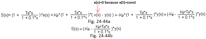

Fig. 24-44
The calculated Laplace transform S(S) of the control signal S(t) shows that for constant x(t) the schemes Fig. 24-44a and Fig. 24-44b are equivalent.
Chapter 24.8.2 The PDy control of a two-inertial object with disturbance z(t)=+0.5

Fig. 24-45
Implementation of the scheme Fig. 24-43b for Kp=10 and Td=5sec.
This is the response of the PDy control, i.e. the PD control with separate differentiation. The signal y(t) very slowly reaches the steady state y=0.91 and barely made it before the disturbance. The controller reacted correctly to the disturbance z(t)=+0.5 by lowering the control s(t). Compare the time chart in Fig. 24-15 with the classic structure of the PD controller. That is, with the version from Fig. 24-43a. Until a disturbance z(t) appears, i.e. up to 30 sec. the system reacts very slowly! And that’s because it was deprived of the differentiating kick from the setpoint x(t) in 3 seconds. Only proportional kick s(t)=10 works, not s(t)=110 as in Fig. 24-15. Then the weakening signal from the proportional component P works (because e(t) decreases). In addition, the differentiating component D brakes powerfully! It stopped braking only after 30 seconds, when y(t) became stable.
Conclusions
In Fig. 24-15 we had a classic version of the PD controller. For it, we selected such settings Kp=10 and Td=5sec so that the respone y(t) was optimal.
We’re getting into a different topic here. What does optimal mean? There are many definitions on this. Intuition should be enough for us. The answer y(t) as quickly as possible with a relatively small one oscillation. The Kp and Td settings, adopted by trial and error, roughly provided us with optimality defined in this way. Another definition may be adopted. E.g. the shortest time chart y(t) without oscillation. It does not swing, but the control time will be longer.
Let’s go back to the conclusions. The settings Kp = 10 and Td = 5 sec in Fig. 24-45 ensured the shortest control time with the setpoint x(t). Even then, it might have come as a surprise that the answer to z(t) was suboptimal. A little long. What it comes from? It’s just that the signal path between z(t) and y(t) is different than between x(t) and y(t). So the input transmittance (between y(t) and x(t)) is different than the disturbance transmittance (between y(t) and z(t)). And this means that settings that are optimal for input transmittance are not optimal for interference and vice versa.
And here we come to the most important conclusion.
1 – When the setpoint value x(t) changes frequently, we use the PD controller version, i.e. Fig. 24-43a
2 – When the setpoint value x(t) rarely changes, we use the PDy controller version, i.e. Fig. 24-43b
Example 1 is a toy-radio-controlled car. The input is the steering wheel, which you have on the control panel with the radio, and the output is the turning angle of the car wheels proportional to the movement of the steering wheel.
Example 2 is a refrigerator. It is often the case that people do not change the set temperature value x(t) for years. This is an extreme example, but in the chemical industry, for example, the setpoint value x(t) changes rarely, while disturbances occur all the time. It is not important to quickly reach the setpoint x(t), but to quickly respond to the z(t) disturbance.
I forgot about the other important plus of the PDy regulator. The time charts y(t) are smooth. The control signal s(t) is also gentler. It may not be so important in the picture, but when, for example, a valve on the pipeline during overregulation constantly “beats the lid” from opening to closing, it will not live long! In the next experiment, we will set the Td setting in the PDy controller due to the optimality of the time charts from the disturbance z(t).
Chap. 24.8.3 PDy control of a two-inertial object with disturbance z(t)=+0.5 with optimal setting TD=1 sec

Fig. 24-46
This is the implementation of the scheme Fig. 24-43b for Kp=10 and Td=1sec. We gave a smaller differentiation Td=1 sec due to the optimal attenuation of the disturbance z(t) (and not the x(t) jump as before).
Probably a faster response to the z(t) disturbance than before. In addition, the response to the jump x(t) improved, although it is not as good as in Fig. 24-43a for the classic PD controller. But for the rarely changing set value x(t) it is not the most important.
Chap. 24.8.4 Comparison of the classic PD control with the PDy control with separate differentiation
Let’s compare the classical PD control optimal for x(t) (which is non-optimal for z(t)) with the PDy control optimal for z(t) (which is suboptimal for x(t)).  A little cloudy, but we know what the author was trying to say.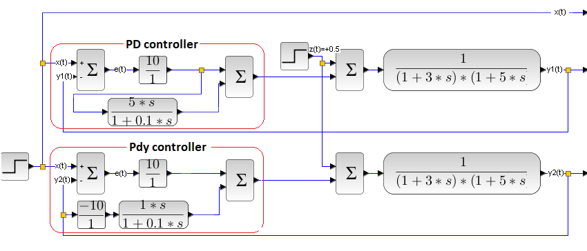

Fig. 24-47
The unit step x(t) simultaneously affects the classical PD control system and the control system with separate PDy differentiation. These are optimal systems due to the setpoint x(t) (upper diagram) and disturbance z(t) (lower diagram).

Fig. 24-48
We only observe the x(t), y1(t) and y2(t). The disturbance z(t)=+0.5 (which is not visible!) will appear in 30 seconds.
Conclusions
1-In the control with separate differentiation of PDy, we are less concerned with the response to x(t) in which changes occur relatively rarely. Therefore, we can focus on optimization due to disturbances z(t) that occur often. So the basic role of the PDy controller is optimal z(t) disturbance suppression, and not optimal (read – nice) reaching the value determined by x(t).
2- An additional advantage of the PDy control is the smoother control time charts s(t).

Chap. 27.9 Conclusions from the PD control
1- Steady state error the same as for the P control. Non zero!
2- Much better dynamic properties than the P control
3- There are PD controllers with error differentiation e(t)=x(t)-y(t) and PDy controllers with only y(t) differentiation.