23. P Control - How does it work?/Jak to dziala?

Automatics

Chapter 23 P Control
Chapter 23.1 Introduction
The length of this and the following chapters on PID is a bit scary. But courage! Most experiments are repeatable with different parameters. The P type Controller is the simplest continuous Controller. In the following chapters, you will learn about more sophisticated PI and PD controllers and the most sophisticated option – the PID controller. They form a group of PID type controllers. It can be said with some exaggeration that the controller is by default a PID controller.
We will examine the control of the P-type regulator with the object:
One-inertial K=1, T1=10 sec.
Two-inertion K=1, T1=5 sec. T2=3 sec.
Three-inertial K=1, T1=5 sec. T2=3 sec. T3=0.5 sec.
Such objects are often found in industry, especially in the chemical industry. Their time constants are of course larger. Each experiment is a response to a step x(t), and then to a step x(t) and a disturbance z(t). The duration is 1 minute for the step x(t) and 2 minutes for the step x(t) and disturbance z(t).

Chapter 23.2 Transmittance Gz(s) and fixed gain Kz of a closed system
This is a short reminder Chapter 16 How does feedback work?

Fig. 23-1
At the entrances of objects
– G(s) in an open system
– Gz(s) or G(s) in a closed system
A unit step x(t)=1(t-3) is given, i.e. a step x=1 with a delay of To=3sec
Open system G(s)
G(s) is a three-inertial object with gain K=10 and time constants T1=1sec, T2=0.5sec and T3=0.1sec. From the G(s) numerator is a gain K=10 in steady state. This amplification as K=y(t)/x(t) from the response to step x(t) confirms the theory. Indeed, in steady state, i.e. after about 20 seconds–>y1(t)=10, x(t)=1. So K=10/1=10.
Closed system Gz(s)
The formula for the transmittance of a closed system Gz(s) and the resulting formula for the steady-state gain Kz are also presented. You will see this in experiments as the steady state output y(t)=y when x(t)=1 . For example, y=0.91 or y=0.99.
Let me remind you that the formula for Gz(s) and for Kz is based on the assumption that the equation K*e(t)=y(t) is satisfied in the steady state.
Then the output signal y(t) tries to follow (more or less exactly) the input signal setpoint x(t), and is immune to disturbances. This is the basis of automatics. If this is not obvious to you, go back to chapter 16.

Chapter 23.3 P controller with a one-inertial object
Chapter 23.3.1 Introduction
The P controller has only one setting – Kp. In chapter 22 (Fig. 22-2d) we have shown that static objects usually have gain K=1. Therefore, the Kp of the controller is also a gain of the entire open system containing the controller and the object.
This approach greatly facilitates the adjusting of the settings of the controller. We will analyze the y(t) response to the x(t) step at various Kp settings. First, let’s examine the object itself. This is where the adjusting of the settings of each controller often begins.
Chapter 23.3.2 An one-inertial object in an open system

Fig. 23-2
The animation confirms that it is an one-inertial unit with K=1 and T=10sec
Chapter 23.3.3 P Control Kp=10
The proportional controller, otherwise the P-type controller, performs the simplest mathematical operation. Namely, it constantly observes the output y(t) and the input x(t) and calculates the control signal s(t):
s(t) = Kp*e(t) = Kp*[x(t) – y(t)]. Here Kp=10.

Fig. 23-3
Response to a x(t) unit step of the controller P when Kp=10
Entire chapter 16 is to repeat ad nauseam that negative feedback systems tend to a steady state where K*e(t)=y(t). And we called the time-varying quantity K*e(t) the goal pursued by y(t). This target is nothing more than the control signal s(t) of the P-type controller.
The calculated K=0.91 is confirmed with the time chart. It can also be justified by simple intuition. The one-inertial unit, which may be e.g. an RC system, will be in equilibrium when s(t)=y(t) and additionally nothing “moves”, i.e. when the time charts s(t) and y(t) are horizontal.
For t=3 sec, the output y(t)=0, because the one-inertial unit (e.g. RC) is “loaded” from 0. Initially, i.e. in 3 sec, the control signal s(t)=10*(1-0)=10. The oscilloscope clips the time charts at level 2 and therefore you don’t see s(t)=10. So RC is loaded at maximum speed. In a “moment” there will be a small positive y(t) and the control signal s(t)=10*[s(t)-y(t)] is a little smaller, and the rate of increase of the signal y(t) will decrease a bit. When will y(t) stop growing? Then when y(t)=s(t). This will happen after approx. 15 seconds.
One more thing. The process is similar to that of the previous chapter when the Client was steering manually. Similar, but not quite. This is due to human imperfection. With more experience with manual controls, the “human” time chart would be more like that.
And if the Client did it precisely by calculating:
s(t)=10*[s(t)-y(t)] every 0.01 sec?
This would get the exact time chart in Fig. 22-3. This is what the Scilab program, which I use for all simulations, did. The Client wasn’t as good at steering as Scilab, but he subconsciously steered as a proportional controller algorithm. At the beginning there was a large error, it gave a large control s(t) signal. The e(t) error decreased, it reduced the control s(t) , until it reached a steady state.
The gain Kp=10 of the proportional controller resulted in:
1. 11-reduction of the gain to Kz=0.91
2. 11-reduction of the time constant to Tz=0.91 sec
This is generally the case for P control. A large Kp causes almost Kz=1 (always a little less than 1!) and increases the speed of the system.
I also propose a full view of the time chart, without the truncated control signal s(t).
You will get exactly the same diagram as Fig. 23-3. What’s the difference? In the (invisible) oscilloscope settings that provide a full view of all signals, especially the control signal s(t).

Fig. 23-4
Unlike the previous animation, you can see how large the control signal s(t) is at the start of the step s(t). The greater the gain Kp of the P controller. Thanks to this, the output s(t) signal at the beginning increases much faster than in the open system in Fig. 23-2. Let’s compare these time charts to appreciate the good job of the P-type controller.

Fig. 23-5
The closed system is 11 times faster. This is an obvious plus of P control. Unfortunately, there was a steady-state error e=1-0.91=0.09. This is typical for Proportional control. The error can be reduced by increasing the Kp gain .
I hope you don’t come to a brilliant conclusion.
An open (without controller) system is slower than a closed system, but its steady-state error is zero!
Indeed, then y(t)=x(t). It’s a holy truth, but a system without controller is vulnerable to disturbances!
Chapter 23.3.4 P Control Kp=100
Let’s also examine the influence of the Kp setting of the P controller on the quality of control

Fig. 23-6
The system is clearly faster and the e(t) error is smaller. In steady state, the red y(t) almost coincides with the black x(t) while the green e(t) is almost zero. This is also confirmed by the theory where approximately Kz=0.99 and Tz=0.1 sec. The oscilloscope clips s(t) at height 2. So let’s see the full time chart with other oscilloscope settings. The diagram will be identical, but with different oscilloscope settings.

Fig. 23-7
Now you see the whole s(t), but x(t), y(t) and e(t) are almost invisible. At high gains Kp, the control signals reach s(t) very large values. For example – a furnace in a steady state requires only 10 kW of power, and at the beginning of the stroke as much as 1 MW! Only a mad designer would give such power. Practically, it will be, for example, 30 kW. Of course, this will adversely affect the time chart, but not as much as 1 MW differs from 30 kW! We will return to the topic in Chapter 31 Influence of Non-linearity on Control
Chapter 23.3.5 Summary of the inertial object controlled by the P controller
It is easy to control. Increasing the Kp parameter will not cause instability or even oscillation, but it will increase the control accuracy. Structural stability at any Kp is easily proved by Hurwitz or Nyquist, whose amplitude-phase characteristic only passes through one quadrant.

Chapter 23.4 P controller with a two-inertial object
Chapter 23.4.1 Introduction
We will repeat the same experiments, but with a two-inertial object. The responds may be more interesting.
Chapter 23.4.2 Two-inertial object in an open system

Fig. 23-8
The object is a serial connection of 2 single-inertial objects with gains K1=K2=1 and time constants T1=3 sec and T2=5 sec. The point of inflection characteristic for multi-inertial systems is visible. Determination of the time constants T1, T2 is not as simple as for the inertial one.
Chapter 23.4.3 P Control Kp=10

Fig. 23-9
The diagram differs from Fig. 23-5 only in another more complicated object.
Also steady state will occur when s(t)=y(t), and “nothing is moving”. So all derivatives are zero. This is after 30 seconds. Unlike the control of the inertial term, s(t) sometimes exceeds y(t). Then s(t) becomes less than y(t), then exceeds y(t) again. And so after a few “pendulums” y(t) will arrive exactly at the calculated fixed value y=0.91. The control signal s(t) has large amplitudes cutted by the oscilloscope. To see the whole s(t) we will repeat the experiment with other oscilloscope settings.

Fig. 23-10
But would you be satisfied with a controller that you set the setpoint x(t)=100ºC and it only gives 91ºC. Unfortunately, that’s the beauty of P-controller. Notice that s(t) is negative at times. So it cools. In order to reach a steady state faster.
There is no zero error e(t). The only thing I can do is increase the Kp of the controller, e.g. to Kp=100.
Chapter 23.4.4 P Control Kp=100

Fig. 23-11
The block diagram obscures the lower e(t) and x(t) signals a bit, but you will see them in the animation.
It is true that in steady state y(t)=0.99*x(t), i.e. y(t) is almost equal to the setpoint x(t), but at the expense of larger overshoots of y(t). In Fig. 23-6, we studied P-control for an one-inertial term and Kp=100. Here we could arbitrarily increase Kp and the system reached the steady state quickly and without overshoots. At large Kp, the fixed error e(t) was almost zero. With a two-inertial term and Kp=100 it is not so nice. Control time and oscillations are unacceptable.
Chapter 23.4.5 Summary of a two-inertial object controlled by the P controller
It is more difficult to control than one-inertial. It can be proved, for example, from the Hurwitz criterion that increasing the Kp parameter will not cause instability. Also with Nyquist which “walks” only in 2 quarters of the open object. Instead, there will be oscillations and a longer calm down time.

Chapter 23.5 P controller with a three-inertial object
Chapter 23.5.1 A three-inertial object in an open system

Fig. 23-12
An one-inertial unit with a time constant T=0.5 sec was added in series to the two-inertial. You will see how such a small change (small To=0.5 sec!) can mess up a feedback system.
Chapter 23.5.2 P Control Kp=10
The system differs from Fig. 23-9 only by an additional one-inertial unit connected in series.

Fig. 23-13
If I proposed such a control to the Client, he would set off the dogs. Not only is there a large error e(t)=0.09, but it dangles after one minute. Increasing the gain to Kp=30 probably won’t improve the situation!
Chapter 23.5.3 Control Kp=30

Fig. 23-14
The system has become unstable. Although the closed-loop gain formula for instability is a bit of a no-brainer, it’s not entirely so. Here Kz=0.97 means that there is a DC component of 0.97 in the oscillation. Let’s see what the oscilloscope cuts off. You will get a diagram exactly the same as in Fig. 23-14. Only the oscilloscope settings are such that the entire control signal s(t) is visible

Fig. 23-15
The scale of the oscilloscope is so small that the unit step x(t) is almost invisible, close to the time axis. However, you can see how y(t) starts to swing, especially the much larger s(t).
Chapter 23.5.4 Summary of the inertial object controlled by the P controller
The hardest to control. The amplitude-phase characteristic of the open system passes through 3 quadrants. Therefore, according to the Nyquist criterion, a closed system may (but does not have to) be unstable.

Chapter 23.6 How does the P controller suppress disturbance?
Chapter 23.6.1 Introduction
Suppression of disturbances is the main job of the controller. There would be no automatics if he couldn’t do it. We previously studied the response to a unit step x(t) that lasted 1 minute. It’s still bearable. But the next experiments will be 2 minutes. First there will be a unit step x(t) and then at 70 seconds a disturbance z(t) (also unit step) positive or negative. It’s like putting an extra heater or cooler into the liquid. The automatics should compensate for this disturbance. That is, with an additional heater, the controller should reduce the supplied power, and with a cooler, increase it. In total, the experiment will last 2 minutes. It’s not much, but some people may find it irritating.
We will examine the P-type control with positive or negative disturbance for previously known objects:
– single-inertial
– two-inertial
– three-inertial
Chapter 23.6.2 Positive disturbance with a one-inertial object Kp=10
We will start with a one-inertial object with a controller Kp=10.

Fig. 23-16
The disturbance z(t) here is additional heating +0.2. As if an additional heater appeared, or the voltage on the heater increased. Up to 70 sec. as in Fig. 26-3. Per disturbance z(t)=+0.2 in 70 sec. controller reacted correctly. He lowered the heating power on the heater behind the controller. Although there is a slight disturbance effect, it has been attenuated 11 times. Complete damping, as you will see later, will only be provided by the integral control e(t) i.e. I, PI or PID.
Compare with the manual control in Fig. 22-16 in Chapter 22. Similar time charts? Yes, only transients are so much better! But with manual control, the steady-state error seems a little less. Weird a bit. Why? Because you subconsciously turned on the I component, which is integration. You reacted to a constant error by gradually slowly reducing the control signal s(t). We will deal with integration in control later.
Chapter 23.6.3 Negative disturbance with a one-inertial object Kp=10

Fig. 23-17
Here the disturbance is negative, z(t)=-0.2. The controller reacted correctly, i.e. with additional heating. But the error is not zero here e=0.09. It can be reduced by increasing the controller gain, e.g. Kp=100. Let’s check it.
Chapter 23.6.4 Positive disturbance with an one-inertial object Kp=100

Fig. 23-18
The oscilloscope cuts the control signal s(t) at the +2 level. But you probably realize that at the beginning of the unit step x(t) the control signal s(t) reaches +100! The greater Kp caused the e error to be almost zero and the reaction almost instantaneous. The system hardly reacts to disturbances.
Chapter 23.6.5 Negative disturbance with an one-inertial object Kp=100

Fig. 23-19
The regulator reacted correctly, i.e. with additional heating.
Chapter 23.6.6 Positive disturbance with a two-inertial object Kp=10

Fig. 23-20
The beginning i.e. the response to the x(t) step is of time chart as in Fig. 23-9. Note that the time scale is different. A bit too much oscillation and long calm down time time. The parameter Kp=10 is not too large and therefore the fixed error is considerable. The suppression of disturbance looks better. Less oscillation and shorter settling time. Often the response to disturbances is more important than reaching the set point x(t). Why? Because the disturbance suppression is continuous, while changes of the setpoint x(t) are less frequent. Nevertheless, it is difficult to present such an arrangement to the client. A bit of a shame about the large fixed error. The experiment is an example that the response to a unit step is different than to a disturbance! This is because the disturbance transmittance Gzakl(s)=y(s)/z(s) is different from the closed-loop transmittance Gz(s)=y(s)/x(s). This is often forgotten when examining the response to a setpoint x(t) and not to a disturbance z(t).
Chapter 23.6.7 Negative disturbance with a two-inertial object Kp=10

Fig. 23-21
Correct reaction. The system tries to compensate for the cooling with additional heating.
Chapter 23.6.8 Positive disturbance with a three-inertial object Kp=10

Fig. 23-22
Even with such a small gain Kp=10, the oscillations and the signal calm down time y(t) are too large. Although it suppressed the “heating” disturbance z(t)=+0.2 by lower control s(t). Fortunately, there is a PD control. We’ll talk about that in the next chapter.
Chapter 23.6.9 Negative disturbance with a three-inertial object Kp=10

Fig. 23-23
No comments.
Fig. 23-14 and 23-15 show that for Kp=30 the system is unstable. Therefore, we will not test the disturbance response z(t) for this Kp
Chapter 23.7 Why is a closed system better than an open one?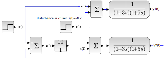

Fig. 23-24
The open-top and closed-bottom systems, which are affected by the following signals:
– input x(t)
– disturbance z(t).
The problem affects all controllers. Not only P-controllers. For many it is a question like why is it better to be healthy and rich than poor and sick? I, for example,prefer healthy and rich.
But if you still have doubts, compare the simultaneous response of the open system y1(t) with the response of the feedback system y2(t) to the input signal x(t) and the disturbance z(t). The controlled and open object will be the previously known two-inertial unit. The regulator is of type P, because we do not know another one yet.

Fig. 23-25
Compare the response y1(t) of the open system and y2(t) of the closed system. Up to 70 seconds, some may still be wondering what they like more. The “open” signal y1(t) takes a little longer to reach x1(t)=1, but without oscillation.
And the most important
y1(t)=x(t)=1!
What cannot be said about y2(t), where the error is as much as 9%! It would seem to be 1:0 for an open system. But the spell disappearsat 70 seconds when negative disyurbance z(t) (cooling) occurs. “Open” y1(t) dropped by as much as 20% and “closed” y2(t) by only 2%.
You can still complain about error of the closed system. Fortunately, automatics has the tools to bring it down to zero. The PI and PID controllers in the following chapters will do this.

Chapter 23.8 Conclusions of P-controller
P-type control
– It is the simplest controllwe from the PID group
– Accelerates the output time chart and suppresses disturbance quickly.
– Does not provide zero error e in steady state. That is, the steady output signal y(t) is always smaller than the setpoint x(t).
– The e error is smaller the higher the controller gain Kp
– For one-inertial units, the gain Kp can be very large. We can then assume that the error is almost zero and the response y(t) is immediate. This approach is also possible for multi-inertial units, when the remaining time constants T1, T2 … Tn are much smaller than the basic time constant T1. Then we treat it “almost” as one-inertial. Instability may occur, but only with very large Kp.
The disadvantage of the P type control is that it requires a larger Kp than PI or PID. And it’s not just oscillations and possible instability. A large Kp causes that at the very beginning the control signal s(t) is, for example, 10 times greater than it is necessary for the output signal y(t) to come to a value close to the setpoint x(t). In the case of water heating, this means that the heater power is also 10 times greater than in the steady state. Also the cables should be bigger.
So far we have assumed that there are no power constraints. In practice, there will always be some, even from the supply voltage. This will result in a slower time charts than ideal. We will come back to this topic in chapter 30.
Generally, in the P control (and not only) there is a basic contradiction of goals. Large Kp is a small control error – great, but also oscillations and even instability. In the next chapter, you will learn that adding a derivative component D to the controller P works like a balm. It “calms down” and allows you to give a larger Kp->smaller control error, although it still does not provide zero error e(t). Then we are dealing with a PD type regulation.