Scilab

Chapter 4.2 First P4-1 program
Rather, it is an opportunity to get acquainted with the Scinotes editor and its cooperation with Console. The program itself is simple.
This is how you do it.
– Copying P4-1 from the course
– Calling Scilab
– Calling the Scinotes editor in Scilab
– Copying P4-1 to the Scinotes editor
– Execute and save P4-1 anywhere*
– Execution of P4-1 on the console in the “with echo” and “without echo” version.
*If you want, you can save it in a specific folder that you create earlier. But this is not necessary. Subsequent programs will be overwritten in this “where you save it” place. Where? It does not matter. After all, you can copy it from the course to the Scinotes editor at any time.
The above steps are shown in the animation Fig. 4-1.

P4-1 program

clear; clc;//Cleaning variables and screen
x=4
y=2
z=x+y
disp(z)

Fig.4-1
How to execute program P4-1 in Scilab?
I advise you to identify all stages very carefully. This is how you will proceed with the next programs. Their operation is similar, so most of them will be without animations.
First, the so-called a program without an echo, then the same program with an echo
The program echoed on the console showing the results of all instructions
The program without an echo showed no response on the console, only the result of the instruction disp(z)
Conclusion
A programmer usually starts testing a program with an echo. He sees what is happening in each instruction.
Then, when it finds errors (so-called debugging), it tests the program without an echo.

Chapter 4.3 Input and Output instructions
After entering the Scinotes editor and executing the P4-2 program, you will know how input instructions of the type x=input(‘Enter data’) and output instructions of the type y=disp(‘data is’, x).

Program P4-2

clear;clc;
x=input('Enter first number ')
y=input('Enter second number ')
z=x+y
disp('The sum is',z)

After meeting the first instruction, i.e. x=input(‘Enter the first number’)*, the program will stop and wait for you to enter a number. It will then save it as x. Remember to click anywhere in the Console window first! Do the same with the instruction y=input(‘Enter the second number’). The instructiont z=x+y is obvious.
Note:
We will only call the program without echo. I don’t know why, but the echo program containing the input instructions doesn’t work properly.
The execution of the program is shown in the animation below.

Fig.4-2
Program with input and output instructions
The figure shows the final state of the animation.
1. Call the Scinotes editor
2. Copy the P4-2 program from the Course
3. Paste P4-2 into Scinotes
4. Click save as… (here we will overwrite as….dokumenty/1.sci) (if you do not save, the program will not execute!)
5. Execute as unechoed file. Remember you are still in the Scinotes editor. So click on the Scilab window to enter data.
6. The message “enter the first number” appeared.
7. I typed 4 and clicked Enter.
8. The message “enter the second number” appeared.
9. I typed 3 and clicked Enter.
10. A message appeared “The sum is 7″.
Carefully analyze the operation of the program. Also Variable Browser states.
The final message where 7 is in the next row is a bit messy. Better would be “The sum of two numbers is 7“
The output instruction must be modified
disp(‘The sum of two numbers is’,z) in which z is treated as a number
for instruction
disp(‘The sum of two numbers is ‘+string(z)) in which z is treated as a string of characters, i.e. text.
Notice that at the end ‘The sum of two numbers is “
there is a space. It will be nicer
P4-3 program

clear;clc;
x=input('Enter first number ')
y=input('Enter second number ')
z=x+y
disp('The sum is '+string(z))

Do this program yourself. Remember to save the program before executing!
Once done you will get something like this.

enter the first number 3
enter the second number 4
“The sum of two numbers is 7”

Chapter 4.4 Instructions related to graphs of two-dimensional functions, i.e. 2D
Chapter 4.4.1 Continuous diagram
We have 2 vectors x and y and we want to graph y=f(x)
Nothing easier.
Just run the following program in Scilab
P4-4 program

clc;clear;
x=[1,2,3,4,5,6,7,8,9,10]
y=[1,4,9,16,25,36,49,64,81,100]
plot(x,y)

The plot(x,y) instruction will connect points with x,y coordinates with straight lines.

Fig.4-3
Continuous diagram plot(x,y)
Remember to save it before executing it. As usual, we will overwrite it on the previous file. Execute without echo. Finally, close the chart window. What for? So that subsequent charts are not overwritten.
Note:
The diahram looks continuous. But if you look closely, he connected the points with coordinates (1,1),(2,4)…(10,100) with straight lines!

Chapter 4.4.2 Dot diagram
What will happen if we replace the plot(x,y) instruction with plot(x,y,’o’)?
The so-called dot diagram is created.

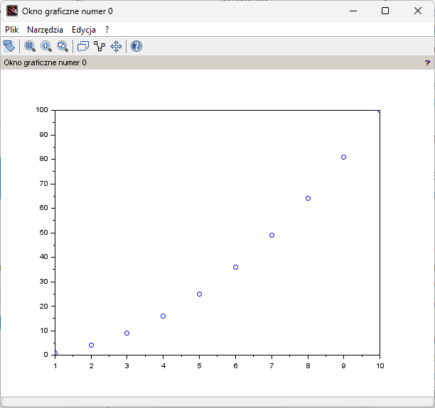
Fig.4-4
Dot diagram plot(x,y,’o’)
Chapter 4.4.3 How to graph any function?
We start from kindergarten, i.e. the graph y=x²

P4-5 program

clc;clear;
x=[-5:0.1:5]
y=x.^2//note the dot next to x
plot(x,y)

The instruction x=[-5:0.1;5] determines the domain of the function y=x². For a mathematician, it is a continuous function for x=-5…+5. In practice, it is a “dense point” chart in the range x=-5…+5 at intervals of Δx =0.1, i.e. for x=-5,-4.9,-4.8….0…+4.8,+4.9,+5.
Note:
The instruction x=[-5:0.1;5] can also be used in another version x=linspace(-5,+5,100). That is, make a graph for 100 equally distributed x variables in the range x=-5…+5.

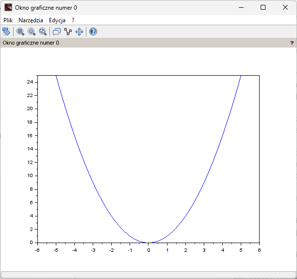
Fig.4-5
Diagram y=x²
Although formally it is a dot diagram, due to the spacing of Δx=0.1, i.e. high density, it is practically a continuous chart.
Try experimenting with the plot(x,y) instruction.
For example, plot(x,y,’–‘) will give something like this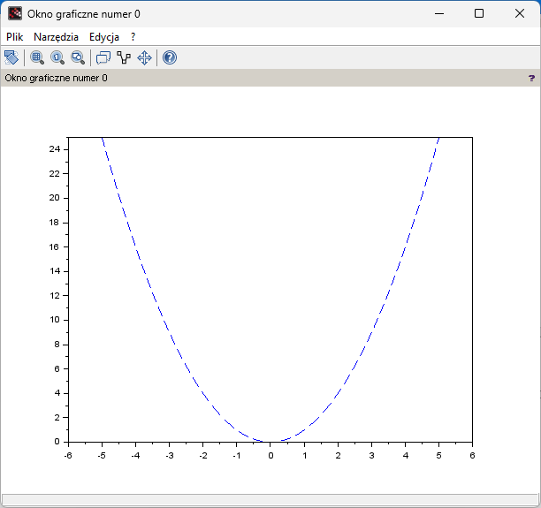

Fig.4-6
y=x² diagram in dashed version.
And we do the colors of the chart like this
plot(x,y) as “default” color blue
plot(x,y,’r’) as color red
plot(x,y,’g’) as color green
plot(x,y,’y’) as color yellow
I suggest experimenting. You will find other colors in “Help” or in other Scilab courses.

Chapter 4.4.4 Texts in the chart
Every decent chart must be described in some way.

Program P4-6

clc;clear;
x=[-5:0.1:+5]
y=x.^2
plot(x,y)
xgrid
legend(['Quadratic function'])
xtitle('Function graph','X-axis','Y-axis')

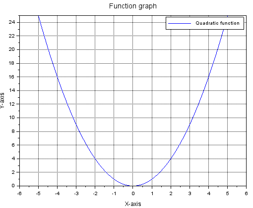
Fig.4-7
The y=x² diagram in the “deluxe” version
– The xgrid instruction in the basic version added a grid. It may also contain additional parameters regarding the mesh itself.
– The legend([‘Quadratic function’]) instruction describes the graph of a function. It would be more important, if there were several graphs on the chart
– The instruction xtitle(‘Graphs of functions’,’x-axis’,’y-axis’) describes a graph and its axes
* The xgrid instruction is in its basic version here.
Scilab allows you to draw 2D charts in any configurations. You can easily place several functions on one chart. E.g. Quadratic and cubic functions. You can also place several charts in one drawing, each containing several functions.

Chapter 4.5  3D charts
Let me just mention that there are such possibilities. At the same time, you will learn how to use sample Scilab programs.

Fig4-8
z=sin(x)*sin(y) as an example of a 3D program
For x=-4…+4 and y=-4…+4
First, you look for this program by clicking the “Examples” icon in the Console window. By right-clicking on the corner of the chart, you can view it from any angle.
Try watching this program yourself in Scilab. Others too