Automatics
Chapter 19. Nyquist Stability Criterion
Chapter 19.1 Introduction
An open system is usually stable. It can become unstable after being closed with a feedback loop. The Nyquist Criterion can predict, based on the amplitude-phase characteristics of an open system (which is “easier” than a closed one), the stability of a closed system. An open system is, firstly, simpler than a closed one, and secondly, it is mostly stable. I mean an open system, so to speak “by nature”, and not one that after applying the formula for Gz(s) becomes “open” as below.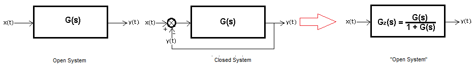
Fig. 19-1
The Nyquist criterion belongs to frequency, unlike the algebraic Hurwitz criterion from the next chapter. The frequency response of an open system is relatively easy to determine as in chapter 18. You can do it on the “living facility” without fear that you will lose control over the industrial installation. After all, it is an open system, and therefore stable. And this is the advantage of the Nyquist Criterion.
Chapter 19.2 Nyquist Criterion
In chapter 18 we got to know the amplitude-phase characteristics. They are fundamental to understanding the Nyquist Criterion. We will examine 3 open dynamical systems, which in Fig. 19-2 have yellow, green, and red amplitude-phase characteristics. They correspond to three successive three-inertial units from Chapter 19.4, 19.5 and 19.6.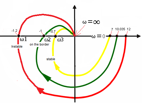
Fig. 19-2
All 3 characteristics apply to open systems.
The inscriptions “Stable”, “On the border” and “Instable” refer to the state, but only after closing them with a negative feedback loop! The characteristic is not to scale. The points on the x axis, i.e. (7.0), (10,035.0) and (12.0) are the numerators of these transmittances, i.e. gains K in steady state. From them “start” individual characteristics with initial pulsation ω=0. In ω1, ω2 and ω3 pulsations, the characteristics pass through the x axis at points x= (-1.2.0), (-1.0) and (-0.7.0). The sinusoids here have a phase shift of φ=-180°. Since these are three-inertial units, they pass through 3 quadrants and for ω=∞ they end at (0,0).
And now the most important, the Nyquist Criterion!
1. If the characteristic doesn’t cover the point (-1.0), then the closed system is stable ->yellow characteristic
2. If the characteristic passes the point (-1.0), then the closed system will be on the border of stability->green characteristic.
3. If the characteristic covers the point (-1.0), then the closed system will be unstable->red characteristic.
Chapter 19.3 Checking the Nyquist Criterion for a stable, boundary and unstable system.
Specific examples will be 3 three-inertial units corresponding to the yellow, green, red characteristics in Fig. 19-2. They will differ only in the numerator of the transmittance G(s), i.e. the gain K=7, 10.035 and 12.
First, we will determine in the most simplified way the amplitude-phase characteristics of a given transmittance G(s) – i.e. yellow, green, red, in an open system. Then we will close them with a negative feedback loop and with the Dirac impulse we will throw the systems out of equilibrium.
Chap. 19.4 Checking the Nyquist Criterion for the transmittance with gain “K=7”.
That is, a stable yellow–>Fig. 19-2
Chap. 19.4.1 Amplitude-phase characteristics of an open system
We should determine the amplitude-phase characteristics for all pulsations in the range ω=0…∞ by feeding sinusoids x(t)=1sin(ωt) of different pulsations to the input. In practice, it is enough for a finite number of ω pulsations. Similarly, we studied, for example, the inertial unit in Chapter 18. Let’s simplify the problem even more. We will limit ourselves only to the ω3 pulsation, in which the characteristic will intersect the x axis at the point (-0.7,0).
The remaining 2 points, i.e.:
(7.0) for ω=0
(0,0) for ω=∞
are derived from Fig. 19-2 and are obvious.
Fig. 19-3
For the pulsation ω3=2/sec (corresponding to the period T=3.14sec), the output sine wave y(t) in steady state is shifted in phase relative to x(t) by φ=-180°. I found the ω3 pulsation by trial and error. The output signal y(t) as a sine wave stabilized after approx. 20 seconds. Only then can its parameters be measured, i.e. amplitude, period and phase. The input sine wave x(t) has an amplitude of 1. Therefore, the amplitude y(t)=0.7 is also a gain for ω3. So K(ω3)=-0.7. The minus sign results from the phase φ=-180°. This means that the yellow characteristic intersects the x axis for ω3 at the point (-0.7.0). So it does not include the point (-1.0) and it is in Fig. 19-2.
Conclusion
The closed system should be stable.
Chap. 19.4.2 Will the closed system be stable?
Fig. 19-4
Three-inertial unit with K=7 in a closed system. The input x(t) is the Dirac pulse. The Dirac impulse knocked the system out of equilibrium, but after several oscillations ω=1.76/sec, the system returned to the state y(t)=0. So the system is stable. The “yellow” characteristic in Fig. 19-2 does not include the point x=(-1.0). This confirms thesis No. 1 of the Nyquist Criterion.
Note:
Initially x(t)=dirac and then x(t)=0. Therefore, almost all the time e(t)=0-y(t), i.e. e(t)=-y(t) in the Fig 19-4.
Chap. 19.5 Checking the Nyquist criterion for transmittance with gain “K=10.035”.
That is, on the stability border-green-->Fig. 19-2.
Chap. 19.5.1 Amplitude-phase characteristics of an open system
We will limit ourselves to the ω2 pulsation, in which the green characteristic intersects the x axis at the point (-1.0). Notice that ω2=ω3=2/sec. This is obvious, because all 3 transmittances differ only in the gain K in the numerator. So for the next transmittance “K=12” there is also ω1=2/sec.
Fig. 19-5
For ω2≈2/sec, the steady-state output sine wave y(t)=1 is shifted in phase by φ=-180° and its amplitude is equal to the input x(t). So K(ω2)=-1. So we have determined 3 important points of the green characteristic for ω=0, ω=ω2=2/sec and ω=∞ as in Fig. 19-2.
Conclusion
The closed system should be on the verge of stability.
Let’s check.
Chap. 19.5.2 Will the closed system be at the limit of stability?
Fig. 19-6
Three-inertial unit with K=10.035 in a closed system.
Input x(t)=Dirac impulse knocked the system out of equilibrium and oscillations of constant amplitude and pulsation ω=2/sec were created. So the system is on the verge of stability. The green characteristic of the open system in Fig. 19-2 intersects the point (-1.0). This confirms thesis No. 2 of the Nyquist Criterion.
Chap. 19.6 Checking the Nyquist criterion for transmittance with gain “K=12”.
That is unstable red–>Fig. 19-2.
Chap. 19.6.1 Amplitude-phase characteristics of an open system
We will limit ourselves to the pulsation ω1, in which the characteristic will intersect the x axis at the point x=-1.2 The other 2 points for ω=0 and ω=∞ are obvious.
Fig. 19-7
“For the pulsation ω1=2/sec, the steady-state output sine wave y(t) is shifted in phase by φ=-180° and its amplitude is 1.2. So K(ω1)=-1.2. So we have determined 3 important points of the red characteristic for ω=0, ω1=2/sec and ω=∞ from Fig. 19-2. This means that the red characteristic intersects the x-axis for ω1 at the point (-1.2.0). That is, it covers the point (-1.0). And so it is in Fig. 19-2.
Conclusion
A closed system should be unstable.
Let’s check.
Chapter 19.6.2 Will a closed system be unstable?
Fig.19-8
Three-inertial unit with K=12 in a closed system.
Input x(t)=Dirac impulse knocked the system out of equilibrium and oscillations of increasing amplitude and pulsation ω=2.14/sec were created. So the system is unstable. The red characteristic of the open system Fig. 19-2 covers the point (-1.0). This confirms thesis No. 3 of the Nyquist Criterion.
Chap. 19.7 Nyquist intuitively
Chap. 19.7.1 Introduction
I don’t know if it will work, but I’ll try. Well, in the Nyquist criterion there is a very characteristic point (-1.0). The stability of a closed system depends on the amplitude-phase characteristics of an open system with respect to this point.
Go back to Chapter 17 Instability, or How oscillations are created.
There was something similar here:
When reinforcement:
K<1, then the closed system is stable
K=1 the closed system is “at the limit”
K>1 the closed system is unstable
We found that the responses to the Dirac of the Delay and Three-inertial unitsare similar, only in the latter the answer is more “fuzzy”. Here again, some simplistic Mr. Nyquist came out, tipping his hat.
So I will try to explain how the true Nyquist Criterion works for the three previously studied three-inertial units:
–”Yellow“
–”Green“
– “Red“
Chapter 19.7.2 Why is “Yellow” stable?
Why the yellow characteristic of the open system in Fig. 19-2 not including the point (-1.0) means the stability of the closed system?
Open system for pulsations ω3=2/s acc. Fig. 19-3 has a gain K=-0.7. The negative sign is the phase shift.
Now look at Fig. 19-4 where negative feedback was used.
The input of the three-nertial is y(t) with reversed phase, because after 3 seconds it is
still x(t)=0 and e(t)=x(t)-y(t)=-y(t)
In turn, we know that for this frequency in a steady state ω=1.76*1/s–>Fig. 19-4, the three-inertial unit almost reverses the phase. Almost … because according to Fig. 19-3 reverses the phase for ω3=2*1/sec.
So the phase is reversed twice, i.e. in a steady state, the sine wave y(t) is in phase with the input signal! Something similar to positive feedback with a gain K=+0.7 in Fig. 17-5 of chapter 17! Since K=+0.7<1, the signal will not sustain itself (as in positive feedback) and the oscillations will disappear. The closed system will be stable.
Chapter 19.7.3 Why is “green” on the verge of stability?
For Yellow, the open system for ω3=2*1/s had K=-0.7. Similarly, for Green, the open system for ω2=2*1/s had K=-1 (Fig. 19-5).
By reasoning similarly to “Yellow”, we will come to the conclusion that the “pseudo-positive” feedback” with the gain K=+1 will cause vibrations with a constant amplitude, as in Fig. 17-7 chapter 17. The oscillations will sustain themselves and the closed system will be on the border of stability.
Chapter 19.7.4 Why “Red” is unstable
Open system gain K=-1.2 (Fig. 19-7). Therefore, a “pseudo-positive” feedback with a gain K=+1.2>1 will cause oscillations with increasing amplitude similar to Fig.17-9 chapter 17. The closed system will be unstable.
Chap. 19.8 Determining the amplitude-phase response from a known transfer function G(s)
In chapter 19.3 we determined the characteristics of the G(s) units with the experimental method by applying a sine wave x(t) with an amplitude of 1 to the input and measuring the amplitude and phase of the output sine wave y(t). We did it for different ω pulsations, theoretically in the range 0…∞. No knowledge of complex numbers was needed. It was enough to interpret the sine wave as a vector of the appropriate length and angle in the x,y plane.
From vectors to complex numbers is very close. Just as a vector has coordinates of the x, y plane, a complex number has coordinates of the P, Q plane, where P is the axis of the real component and Q of the imaginary component. Operations known in “ordinary” mathematics are also performed on complex numbers. Addition, subtraction, multiplication and division. There are appropriate formulas for this and that’s it. So, knowing them, you can determine the amplitude-phase characteristics of a given G(s). Substitute s with the imaginary number jω, where ω is the appropriate pulsation and the complex number G(jω) will show us the appropriate value for the pulsation ω.
Let me remind you that G(s) is a fraction of two polynomials of the numerator L(s) and the denominator M(s). For this, we only need monkey dexterity to perform 4 basic mathematical operations on complex numbers. The amplitude-phase characteristic calculated in this way for various ω pulsations will look similar to the previous one:
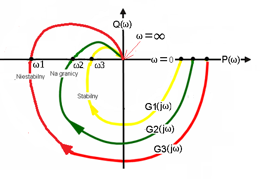
Fig.19-9
The amplitude-phase characteristic G(jω) calculated from the transmittance G(s).
G(jω) is the so-called spectral transmittance. It contains the same information about the static and dynamic properties of the object as the operator transfer function G(s).
Conclusion:
All pulsations ω1, ω2 and ω3 in Fig. 19-2 were the same, i.e. ω1=ω2=ω3=2/sec. But only because the transfer function denominators G1(s), G2(s) and G3(s) are the same! This is usually not the case and therefore usually ω1, ω2 and ω3 are different.