Scilab

Chapter 13 XCOS-How Does Negative Feedback Work?

Chapter 13.1 How does Feedback Work?
In Automatic Control Systems, the most important thing is to understand the principle of Feedback. It must be as obvious and intuitive as riding a bike! Occurs when the output signal y(t) returns back to the input.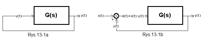

Fig.13-1
Fig. 13-1a
The signal y(t) from the output returns directly to the input. But what is the cause and what is the effect? Did the egg come first or the chicken? Not to mention more existential questions. So let’s treat the diagram as a curiosity.
Fig.13-1b
This means some contact with the outside world is needed. This is done by calculating the difference e(t)=x(t)-y(t) in the so-called comparison node. This is the most important scheme in automatics because y(t) tries to mimic x(t). That’s why you need to understand it well!

Chapter 13.2 How does positive feedback with the Inertial System work?
The input is given the sum of the signals e(t)=x(t)+y(t) instead of the difference as in Fig. 13-1b. It is easier to understand than negative feedback and that is why we analyze this case.
Note:
1. The SUMMATION block in the simulation below can be found in the Mathematical Operations palette.
2. A short impulse x(t) (“disruption”-a substitute for the Dirac impulse) in 5 seconds can be realized, for example, as the difference of step units shifted in time by 0.01 sec ->2(t-5) and 2(t-5.01).

Fig. 13-2
The input of the inertial unit is the sum s(t)=x(t)+y(t). Initially x(t)=y(t)=0. So s(t)=0+0 =0 and nothing happens. But at the fifth second, a “pin” appears. Just a little disturbance. This signal will pass through the inertial unit as a “damped spike” with lower amplitude and magnified by a factor of 1.5. At first this “damped spike” is so small that it doesn’t show up on the chart, but it will immediately come back to the input and be increased again by 1.5 times. It will come back again and again be increased by 1.5 times…etc. Classic avalanche effect. The system was unstable from the very beginning, although it was not visible until the fifth second. But a small “spike” was enough for a disaster to occur.
Note:
Positive feedback is not always unstable as in Fig.13-2. For example, try K=0.8 instead of K=1.5. Just reduce Ymax on the oscilloscope from 10 to 0.1 to increase the gain of the oscilloscope. After the “spike“, the system will reach the steady state y(t)=0. Note that now o<K<1, unlike Fig.13-2 when K>1! If you had given a step unit instead of a “spike“, the output y(t) would have reached y=4.

Chapter 13.3 How does negative feedback with the Inertial System work?
That is, how the inertial unit with negative feedback reaches the steady state. This applies to any blocks in an open system (i.e. without feedback), which give a finite value in response to a unit step. That is, the so-called static system. I advise you to thoroughly understand the principle of achieving a certain balance. This is the basis of automatics. Especially since most authors approach it purely mathematically. The calculations show that there will be some steady-state error e=x-y. I.e. difference between the set setpoint x and the output y.

Fig.13-3
Inertial unit with negative feedback.
The signals shown on the oscilloscope are:
– output y(t)
– goal K*e(t) (K=5)
The signal y(t) tends to the goal K*e(t), which varies in time. The “driving force” that tries to bring the goal K*e(t) and y(t) closer together is also the difference U=K*e(t)-y(t) in the form of a vertical green line in the right figure. The greater the difference U – the “driving force”, the stronger the lines K*e(t) and y(t) “cling” to each other.

The output y(t) tends to the equilibrium state y(t)=K*e(t) in which the “driving force U” disappears – the vertical green line
And when will y(t) stop growing? Or in other words – when will there be a steady state? Then, when the goal is achieved, when the driving force (vertical green line U) disappears! That is, when y(t)=K*e(t).
This is true not only for the inertial unit, but for any dynamic unit with negative feedback, which in the steady state has a gain K. The experiment confirms something very important in automatics. Just as a pendulum thrown out of balance will return to its steady state, which is its lowest position
Thus, a stable system with negative feedback will return to the state y(t)=K*e(t)
The above equation, i.e. y(t)=K[x(t)-y(t)] after ordinary school transformations results in y(t)=K*x(t)/(K+1)*. That is, for a very large gain K and in steady state y(t)≈x(t). That is, the output y(t) tries to imitate the input x(t). This is the most important goal of automatics,
The inertial unit is an example of the so-called static object. I.e. one that does not have an integrating unit. Here, understanding the principle that “output y(t) tries to imitate input x(t)” was not the easiest. Unlike the so-called astatic objects in which the output y(t) in the steady state is perfectly equal to the input x(t). You will find out in chapter 13.4.
*Just in case, I will show these transformations in Chapter 13.5

Chapter 13-4 How does a negative feedback integral term reach its steady state?
If an object, e.g. an integrating unit with inertia, has an integrating unit, it is called an astatic unit. All the more so it will be a “pure” integrating unit.

Fig. 13-4
You see how the integrating unit reaches the steady state y(t)=x(t)=1. Compare with Fig. 13-3 with the inertial unit which is static. In it, the “driving force” that strives for a state of equilibrium was 5*e(t)-y(t). Here, however, the driving force is the error e(t). Simplicity is beautiful!
When x(t)>y(t) (or e(t)>0) then y(t) increases as in any decent integrating unit. I will also add that it is growing at a decreasing speed because e(t) is constantly decreasing. In the steady state, this speed is, of course, zero. Then y(t)=x(t)=1 and e(t)=0

Chapter 13.5 Conclusions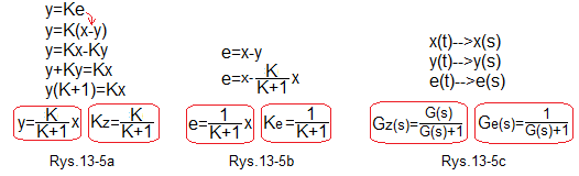

Fig.13-5
Relationship between input, output and error.
Fig.13-5a
The relationship between y and x and the gain Kz of a closed system in the steady state.
Fig.13-5b
The relationship between the error e and x and the error gain Ke of a closed system in the steady state.
Fig.13-5c
The relationship between the transforms of the input x(s), output y(s) and error e(s), as well as the transmittance of the closed system Gz(s) and the error Ge(s). From them, you can obtain time graphs y(t) and e(t).
Conclusions
The equtions in Fig. 13-5 are universal. They concern systems with and without integrating units, i.e. astatic and static systems.
What is the gain in the steady state at the step unit of an astatic system, i.e. one containing an integrating unit? At the input x=1 and at the output y=∞ (infinity). So K=∞.
Then formula 13-5a will transform into y=x and Kz=1 and formula 13-5b will transform into e=0 and Ke=1
This means that a closed system containing an integrating unit can provide zero error in the steady state. That is, a state in which the output y “obeys” the set value x.