Automatics
Chapter 8 Integrating Unit with Inertia
Chapter. 8.1 Introduction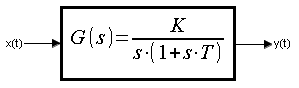
Fig. 8-1
Transmittance of the integral unit with inertia.
Do you remember the integral unit? The step x(t) at the input caused the output signal y(t) to increase to infinity with a constant speed. I emphasize. With a constant speed from the beginning of the step x(t).
The integral unit with inertia also tends to infinity. But he does it a little differently. At the beginning of the step, x(t) “accelerates” starting from a velocity V=0 and ending with a certain fixed V=const. So it is a more accurate approximation of, for example, an actuator than a ideal integrating unit.
Chapter 8.2 k=1 T=3 sec with slider and bar graph
Again, we’ll start with the bargraph to get you acquainted with the dynamics.
The inertial unit is a series connection of the integrating 1/sTi and the inertial 1/(1+sT). Here Ti=1sec and T=3sec
Fig. 8-2
The slider is initially set to 0. I gave it x(t)=+0.1=max. You will observe waveforms similar to those for the previously tested integrating unit. You also need to give 0 to the input to stop the y(t) output signal. A digital meter will be useful for the 0* setting. If you managed to stop y(t) (does not increase or decrease), then a typical feature of PI or PID controllers will be revealed. The fixed output of the yr(t) controller is different from zero, although the input is zero!
The waveforms are similar to the integral unit, but not the same! I hope you can see the inertia. Especially when you enter +max and in a moment -max. You will notice that the signal continues to increase for a short time even though x(t)=0 and even decreases! The phenomenon of inertia will be clearer in the next experiment with the oscilloscope.
*It is difficult to set an exact 0 on a digital meter. Rather, it is a signal close to 0, e.g. x(t)=+0.002. This means that y(t) will “almost stop” i.e. y(t) is increasing very slowly.
Chapter 8.3 Ti=1 sec and T=3 sec with jump and oscilloscope
The integrating unit with inertia is a series connection of the integrating unit 1/sTi and the inertial unit 1/(1+sT). Ti=1sec and T=3sec.
Fig. 8-3
The input is a step x(t)=1. The signal yp(t) is after the integrator, y(t) is the output. At the beginning, the inertia T=3 sec is clearly visible. In the steady state, both signals grow at the same speed. The integrating unit with inertia is an example of the so-called astatic system. At non-zero x(t), the signal y(t) increases or decreases. For this integrating unit Ti=1 sec as the time after which yp(t) becomes equal to x(t). This is also the time after which, in the steady state, y(t) will increase by the step value x(t)=1, i.e. Ti=1 sec.
In steady state, i.e. after approximately 18 sec, the output signal y(t) is delayed by T=3 sec.
Chapter 8.4 Ti=1 sec T=3 sec with a single square pulse and an oscilloscope
The inertial integrating unit is acted upon by a single rectangular pulse.
Fig. 8-4
This is a more accurate approximation of the actuator – a motor with a gearbox as an ideal integrating element whose arm can control the valve position. This example is discussed in Chapter 4. Integrating Unit. Here, however, we also take into account inertia. The black x(t) input is the voltage at the motor and the red output y(t) is the valve stem position. Needless to say, inertia, consisting mainly of mechanical inertia + some electrical inertia – inductance, “spoils” the quality of the device. In an actuator, it would be difficult to extract the yp(t)-signal directly after the integrator. This is only possible in the model as in Fig. 8-4.
Chapter 8.5 Integrating Unit with inertia k=1 T=1.25 sec with positive and negative rectangular pulse and oscilloscope
We will see how the actuator works by “searching” for its position.
I.e. it turns once in one direction and once in the other until it finds the position set by the regulator and stops. Therefore, the inertial integrating unit is acted upon by a positive and negative rectangular impulse.
Fig. 8-5
The blue yp(t) is an ideal actuator without inertia. The red y(t) is the real actuator. The actuator from Fig. 8-4 with inertia T=3 sec was bought by a poor customer. Now the client is Lord, who wants the actuator to respond quickly. That’s why I sold the actuator with lower inertia T=1.25 sec. The effects are visible. The actuator will reach the set speed faster. Therefore, it will also reach the set y(t) faster. First, a positive pulse set the valve to y(t)=8, the actuator stood for a while (because that’s what e.g. the regulator wanted) and then a negative pulse set the valve to y(t)=4.