Automatics
Chapter 9 Differentiating Unit with Inertia
Chapter. 9.1 Introduction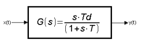
Fig. 9-1
Transmittance of the Differentiating Unit with Inertia.
Do you remember the ideal differentiator in Chapter 5? The linearly increasing signal x(t) at the input caused a step y(t) at the output with an amplitude proportional to the rate of increase x(t). The Differentiating Unit with Inertia works similarly. It also measures the rate of increase x(t), but it does so with some inertia. It can be said that calculating the rate of increase x(t), i.e. calculating the derivative y(t)=x'(t) will take him some time. Not so immediately as in ideal
Chapter 9.2 Differentiating Unit with Inertia Td=2sec T=0.5sec, sawtooth with oscilloscope
Fig. 9-2
Differentiating Unit with Inertia Td=2 sec T=0.5 sec.
For this unit test with, the best solution is x(t) increasing linearly with the speed (derivative!) 1/sec. The formula for x(t) is given in the diagram. Check if it is correct, e.g. for t=0 and t=7 sec. The output signal calculating the speed x(t) settled down after about five time constants T, i.e. after 5*0.5 =2.5 sec. So T proves the quality of the speedometer. A cheap speedometer will give you the exact speed after, for example, 2.5 seconds, as in the example, and a good one after, for example, 0.5 seconds. And what is Td=2 sec? Go back to the ideal differentiator for a moment–>chapter 5, i.e. without inertia. There Td=1 sec and it was the time after which the output y(t) equaled the saw x(t). Here the definition is similar, only it applies to a steady state, e.g. after 3 sec. Here, after Td=2 sec, the signal increment x(t) also equals y(t)=2. Note that the larger the Td, the greater the differentiation intensity.
Chapter 9.3 Differentiating Unit with Inertia Td=2, T=0.5 sec, rectangular pulse with oscilloscope
Fig. 9-3
Instead of a saw, there is a rectangular pulse at the input
Compare this waveform with the analogous one, only for the ideal differentiating unit ->Fig. 5-9 chapter 5. There, at the positive slope of the step x(t), the speed y(t) was infinitely large. Ideal showed this as a Dirac impulse. Here, the real one showed y(t) as a rate of 4/1sec when t=3.5sec.
From the plot y(t) we can obtain the parameters of the differentiator:
– T=3.5-3=0.5sec (from the green tangent)
– Td=4/05sec=2/sec
Conclusion-rectangular pulse has more difficult interpretation than a ramp.
.