Automatics
Chapter 26. PI Control
Chapter 26.1 Introduction
From chapter 25.8 of the previous chapter, we learned that:
– P Control, and even more so PD, reacts quickly to the setpoint x(t), but does not provide steady error e(t)=0.
– With type I Control it is the other way around. The system slowly approaches the setpoint x(t), but it provides a steady error e(t)=0.
Therefore, the idea of a PI controller with a proportional P unit and an integrating I unit suggests itself. We expect its response to a setpoint x(t) and a disturbance z(t) to be faster than that of the I controller (although not as fast as P or PD!), but in steady state the error e(t) will be zero. We will start by studying the structure of PI. This is not yet a PI controller but a PI unit because the input is only a single signal x(t) and not the error e(t)=x(t)-y(t).
Chapter 26.2 PI unit
Chapter 26.2.1 PI unit Kp=1 Ti=1 sec
Fig. 26-1
Kp=1 Ti=1 sek
The input signal is the unit step x(t). The proportional component yp(t) and the integral component yi(t) are clearly visible. The component yp(t) is for Kp=1 a repetition of the jump x(t). The component yi(t) is an increasing “ramp” for which the value after time Ti=1sec is also yi(t)=1. The controller signal y(t) is then twice the value of the initial signal y(t). Hence another name for the integration time Ti is the doubling time Ti. With the same Ti and different Kp of the PI controller, the slew rates of the output signal y(t) are different, but their parameters Ti will of course be the same.
Chapter 26.2.2 PI unit Kp=1 Ti=10 sec
Fig.26-2
Kp=1 Ti=10 sec.
It integrates 10 times slower than before, but after Ti=10 sec the output signal is also doubled.
Chapter 26.2.3 PI unit Kp=3 Ti=10 sec
Fig. 26-3
It integrates 3 times faster than before, but after Ti=10 sec the output signal is also 3 times bigger. But the Kp setting has no effect on Ti.
Chap. 26.3 Control system with Didactic PI controller
Chap. 26.3.1 Didactic PI controller
The didactic PI controller that I tinkered with will show that the component:
– proportional P for faster operation
– integrating I ensures zero error
– at unit step x(t) starts as proportional P and ends as integral I. This transformation will occur at some point. In a real PI controller, the transformation P–>I occurs continuously. You’ll find out later.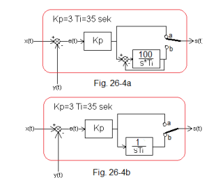
Fig. 26-4
The structure of the controller depends on the position of the contact:
-Fig. 26-4a-contact “top”
P-type structure. Note that at this time at contact b, thanks to the strong negative feedback involving the integrating unit, the voltage at contact b follows the voltage at contact a. If you don’t believe it, put G(s)=100/sTi to the most important formula in automation –> Fig. 15-3d chapter 15.
-Fig.26-4b-“down”contact
-type I structure. Thanks to the above-mentioned tracking, after switching from contact a to b, the system will behave as in the animation in Fig. 26-5
Fig. 26-5
Up to 25 seconds, the controller is P-type and y(t)=Kp*e(t)=3*1=3. In the 25th second, the contacts drop (you can see it in the animation) and the controller becomes type I. Thanks to “tracking”–>Fig. 26-4a, the integration starts from +3V and not from 0V. After the so-called at the doubling time Ti=25 sec, the I component equaled the P component. If, for example, in 40 sec. if the error e(t) increased a little bit, then s(t) would start to grow like a dashed line. There will be no signal spike s(t) because only the integral component I acts.
Chapter 26.3.2 Control system with didactic PI controller
We will show that the component:
-proportional P is responsible for a quick approach of y(t) to a state close to the setpoint x(t)
-integrating I is responsible for reaching the state in which y(t)=x(t). So it will provide steady error e(t)=0.
After that, it will be easier for you to understand the operation of a real PI controller.
Fig. 26-6
Didactic PI controller with settings Kp=10 and Ti=50sec was used.
Before 12 sec, only the proportional component P works, and after 12sec, the integral component I.
Before you press the video button, take a good look at the signals:
–control blue s(t)
–output red y(t)
– green error e(t)
In 12 seconds, the structure of the controller changed from P to I, i.e. the contacts from a to b were dropped.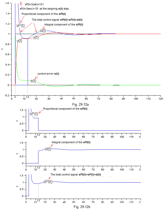
Fig. 26-7
Fig. 26-7a shows all the time charts. The control signals sP(t), sI(t) and sPI(t) overlap and therefore Fig. 26-7b was created, where these signals are shown separately. Here it is clear that in 13 sec the proportional component sP(t) disappears and the integrating component sI(t) appears. The total signal sPI(t) is the sum of the components sP(t) and sI(t). Due to the different scales, the time charts in Fig. 26-12a and Fig. 26-12b are not identical.
In 3 seconds, a unit step x(t) occurred. Then the control signal is only the proportional component sP(t) and the output signal y(t) will very quickly reach the steady state y=0.91. Certainly faster than if only the I controller was working. In 12 sec. the controller changes its character from P to I and since then only the integrating component sI(t) is active. We know very well that it can reduce the error e(t) to 0, which it does willingly. Therefore, after about 90 seconds x(t)=y(t)=1 or e(t)=0.
Short and to the point.
In PI control, the P component quickly brings the output signal y(t) to a signal close to the setpoint x(t) (but smaller) here to y(t)=0.91. P-control is unable to bring the steady-state signal y(t) to y(t)=x(t).
The didactic controller knows this handicap and therefore switches off sP(t) and switches on sI(t) in 12 seconds. And the integrating component sI(t) will lead the signal y(t) to the value y(t)=x(t)=1 after some time, i.e. it will ensure zero control error.
Chap. 26.3.3 Comparison of didactic PI with P-control
See Fig. 26-7a. The P-type controller is a special case of the didactic controller, in which there will never be a switch from P to I. That is, after 12 sec. the same state y=0.91 will remain. Compared to the didactic PI controller, the error of the P-type control is not zero.
Chap. 26.3.4 Comparison of didactic PI with Type I control
The I-type integral controller is optimal for a single-inertial object with a time constant T=10 sec, when its setting Ti=16 sec. Let’s compare this control with the didactic PI.
Fig. 26-8
For 2 control systems with an one-inertial object controlled by the:
– didactic PI controller
– classical I controller (integrating)
the same unit step x(t) is given. Both controllers should reduce the steady error e(t) to 0. Which will do it better? i.e. faster and with less oscillation. 5:0 for didactic PI! It comes to a steady state y(t)=1 faster and with less oscillation than type I control. You will soon see that real (not didactical) PI control is even better!
Chapter 26.4. PI controller with one-inertial object
Chapter 26.4.1 Introduction
Time for a “real” PI controller, which is simply a PI controller.
This topic in chapter 26.4, 26.5, 26.6 are PI controllers for objects:
–single-inertial,
-two-inertial,
-three-inertial.
We will study control systems with different Kp and Ti settings. We will always start with the integration action turned off, and then the PI controller will become a P controller. Why? Because you will see the main advantage of the PI controller. Reducing the control error to e(t)=0 while operating much faster than the I controller.
Chapter 26.4.2 One-inertial object
Fig. 26-9
One-inertial object with time constant T=10 sec K=1
By the way, you will remember how to read the parameters of an one-inertial object K=1 and T=10 sec from the time chart.
Chap. 26.4.3 PI control Kp=3 integration disabled
So we have a typical P-type control. Kp=3 disables integration (0 in the numerator of the integrating unit I disables integration).
Fig. 26-10
Up to approx. 19 sec., the control works as PI didactical control up to 12 sec. in Fig. 26-6. So it is a P-type control. It is true that Fig. 26-6 shows a different Kp, but it does not prevent us from analyzing. The output signal reached after 19 sec. steady state y(t)=0.75 and this is consistent with the time chart and the theory for P-type control. So there was a non-zero error e(t)=0.25. In order to eliminate the non-zeroness of the error e(t), let us introduce an integrating component I. We will start with a careful (“slow”) integration of Ti=12 sec.
Chapter 26.4.4 PI control Kp=3 Ti=12 sec
If you want to remember how the PI unit reacts to a step x(t) in an open system, go back to chapter 26.2. After adding the I component, the P controller became a PI controller. Will the error e(t) be set to zero?
Fig. 26-11
Yes, yes, yes!!! After about 50 seconds), the red y(t) coincided with the black x(t). So the error e(t)=0. Such a quite good time chart was obtained with quite careful settings, low Kp and high Ti. We expect that with more “aggressive” settings, the system will reach the steady state y(t)=1 faster. Perhaps at the expense of oscillation, because nothing in life is free.
Chapter 26.4.5 More detailed analysis of the PI Regulation Kp=3 Ti=12 sec
Let’s try to find an analogy with the already well-developed PI didactic controller, i.e. with the time chart in Fig. 26-6. Same control system as before. But now we study not only the control signal of the sPI(t) controller, but also its proportional component sP(t) and integrating component sI(t).
Fig. 26-12
The didactic PI controller in Fig. 26-6 starts the action as (only) proportional P. This allows it to reach a steady state y(t) very quickly. Let me remind you that in the P control at the beginning of the the control signal sPI(t) is very large and this is what forces a time chart. Then, when the steady state is reached (which is always less than x(t)=1), the I integral action is switched. Now the I integral controller will do what it does best. It will complete the action, i.e. it will bring the control error to e(t)=0. The red y(t) will coincide with the black x(t).
And how does a “real” PI controller in Fig. 26-12 do this?
Similarly. At the beginning of the step x(t) only the proportional component sP(3)=3 is active, because the integrating sI(t) “has not yet grown up” (sI(3)=0). As in didactical unit.
And in a steady state, e.g. in 55 seconds?
Here it is the opposite, only the integrating component sI(t) works because the proportional one has disappeared – sP()=0. Just like in didactical too.
And between t=3 sec and t=55 sec?
Then sP(t) disappears and sI(t) increases. So, to use elegant words, the P controller changes into the I controller. In a continuous manner, not stepwise as the didactic PI controller! That’s it. Are there questions? I do not see. So let’s do a more aggressive (or faster) integration. Hopefully this will speed up the time chart without exaggerating the oscillation.
Chapter. 26.4.6 PI control Kp=3 Ti=4 sec
More aggressive integration will certainly speed up the time chart, but at the expense of large oscillations?
Fig. 26-13
The scope of the oscilloscope has since changed. It was 0…3, it’s -1…2. The scale remained the same. Change due to appearance of negative e(t).
Faster runs compared to Fig. 26-12 when Ti=12sec. The steady state is already after approx. 25 sec. at the expense of some control time. Some may like the previous Ti=4 sec better. But let’s assume that our client’s priority was the time to reach a steady state. Even at the expense of the appearance of oscillations. How about an even faster integration?
Chapter. 26.4.7 PI control Kp=3 Ti=2 sec
Fig. 26-14
I think we overdid it. Large oscillation and control time similar to the previous one. So far we have studied the system by changing Ti when Kp=3. We will continue to do the same, but with Kp=10. We expect faster time charts and larger oscillations.
Chapter 26.4.8 PI control Kp=10 without integration
We’ll start with a non-integral control. that is, from the type P control.
Fig. 26-15
From the time chart and theory, for the proportional control when Kp=10, the output signal y(t) in the steady state is y=0.91 and the error e=0.09. In Fig. 26-16 is the same time chart, but on a different scale. You’ll see the entire “unclipped” control signal s(t).
Fig. 26-16
This control signal s(t) is large.
In order for the steady error to be zero, the integration must be turned on.
Chapter 26.4.9 PI control Kp=10 Ti=15 sec
Fig. 26-17
Better than Kp=3 and Ti=4sec in Fig. 26-13. So let’s increase the intensity of the integration even more.
Chapter 26.4.10 PI control Kp=10 Ti=5 sec
Fig. 26-18
I guess it’s better. There is a slight overshoot, but the steady state came much faster. We will increase the integration again.
Chapter 26.4.11 PI control Kp=10 Ti=1.75 sec
Fig. 26-19
If we care about the control time and the overcontrol of about 20% is not a problem, then the settings Kp=10 Ti=1.75sec are the best for our one-inertial object. Otherwise, Kp=10 Ti=5sec are optimal. Of course there could be even better settings. Only the responses with other combinations of Kp and Ti need to be investigated.
Now let’s move on to looking for the optimal setting for a slightly more difficult to control object – Two-inertial.
Chapter 26.5 PI controller with two-inertial object
Chapter 26.5.1 Two-inertial object
Fig. 26-20
Two-inertial object with time constants T1=3 sec, T1=5 sec, K=1. You see a point of inflection typical for multi-inertial units.
Chapter 26.5.2 PI control Kp=3 integration disabled
So we start with the P control.
Fig. 26-21
The output signal reached after 35 sec. steady state y(t)=0.75, and this is consistent with the time chart and the theory for P-type control. There was a non-zero error e(t)=0.25. To make th e(t)=0, let us introduce an integrating component I. We start carefully with Ti=32 sec.
Chapter 26.5.3 PI control Kp=3 Ti=32 sec
Fig. 26-22
The error signal e(t) reaches the zero state. The chart doesn’t show it,because the time of the experiment was too short.
Chapter 26.5.4 PI control Kp=3 Ti=8sec
Fig. 26-23
Here we have already reached the steady state when e(t)=0. It got better. Let’s move on
Chapter 26.5.5 PI control Kp=3 Ti=5 sec
Fig. 26-24
We went a bit overboard with the intensity of the integration. It was better before.
Chapter 26.5.6 PI control Kp=10 integration disabled
Fig. 26-25
Steady state consistent with the theory for P control, i.e. e(t)=0.
Chapter 26.5.7 PI control Kp=10 Ti=20 sec
Fig. 26-26
At 60 seconds, the error is not yet zero. Let’s reduce Ti. Note the oscillation amplitude of the control signal sPI(t) compared to the output signal y(t). It is generally larger.
Chapter 26.5.8 PI control Kp=10 Ti=10 sec
Fig. 26-27
Not bad. But the setting Kp=3 Ti=8 sec from Fig. 26-23 is better for a controlled two-inertial object. And we’re used to the fact that a large Kp is mostly good. Let’s reduce Ti further. Will it help?
Chapter 26.5.9 PI control Kp=10 Ti=5 sec
Fig. 26-28
Did not help. Too much oscillation.
Now let’s move on to the most difficult object – the three-nertial one.
Chapter 26.6 PI controller with three-inertial object
Chapter 26.6.1 Three-inertial object
Fig. 26-29
Three-inertial object – K=1 and time constants T1=0.5 sec T2=3 sec, T3=5 sec.
At first glance, it is difficult to distinguish from a two-inertial one.
The more inertia (here T1, T2 and T3) the more clearly the delay parameter is marked – here To=1.3 sec.
Chapter 26.6.2 PI control Kp=10 integration disabled
Fig. 26-30
Steady state, i.e e(t)=0, consistent with the theory for P-regulation.
Chapter 26.6.3 PI control Kp=10 Ti=16 sek
Fig. 26-31
The output signal slowly reaches a steady state y(t)=1. So let’s increase the to Ti=10 sec.
Chapter 26.6.4 PI control Kp=10 Ti=10 sek
Fig. 26-32
Increasing the integration rate had the desired effect. After 45 sec. the condition x(t)=y(t) occurred, i.e. e(t)=0. Let’s reduce Ti further.
Chapter 26.6.5 PI control Kp=3 Ti=4 sec
Fig. 26-33
It is worse. And what will happen when we increase Kp?
Chapter 26.6.6 PI control Kp=10 integration disabled
I,e P control.
Fig. 26-34
According to the theory, for a steady state of P-type control, after 60 seconds, a steady state will occur y(t)=0.91 and e(t)=0.09. In order to bring the control error e(t) to 0, we will start with a cautious (i.e. slow, i.e. large Ti) integration.
Chapter 26.6.7 PI control Kp=10 Ti=16 sec
Fig. 26-35
The y(t) oscillations occur around x(t)=1. Finally in agony after 60 sec. control error will be zero. So let’s reduce Ti to make it faster.
Chapter 26.6.8 PI control Kp=10 Ti=8 sec
Fig. 26-36
It is worse. So for this three-inertial object, the optimal PI control settings are Kp=3 and Ti=10 sec from Fig. 29-60. We got used to Kp=10 giving better results than Kp=3. So it’s not worth getting into habits, especially in automation. And what will happen when we increase the integration intensity to Ti=2.5 sec?
Chapter 26.6.9 PI control Kp=10 Ti=2.5 sec
Fig. 26-37
Notice the unusual scope of the oscilloscope. Although it is an unstable system, up to 3 seconds nothing happens at the output because nothing happens at the input. In 3 seconds we “knocked” the system with Dirac pulse, bringing it out of equilibrium in this way.
Chapter 26.7 PI control with disturbances
Chapter 26.7.1 Introduction
The same one-, two- and three-inertial objects will be controlled. Their inputs will be affected by input signals x(t) (as before) and disturbances signals z(t)=+0.5 or z(t)=-0.5. Disturbances will cause an error e(t) which will “annoy” the PI controller so much that it will always bring it to 0. More precisely. The proportional component P will bring the error e(t) to a value close to 0 and the integrating component I will finish the job bringing it to 0. The experiment will last 2 minutes. The settings that gave the “prettiest” response in previous experiments will be used. The “prettiest” i.e. relatively fast and with possibly small oscillations. Let’s call these settings optimal, although they can be even better. After all, we studied only a few combinations of Kp, Ti.
Chapter 26.7.2 Positive disturbance with a one-inertial object z(t)=+0.5 Kp=10 Td=5sec
The disturbance z(t)=+0.5 will occur in 70 seconds.
Fig. 26-38
Up to 70 seconds, i.e. until the appearance of the disturbance, the time chart is the same as in Fig. 26-18, taking into account the different time scale on the oscilloscopes. Initially, the disturbance z(t)=+0.5 caused the signal y(t) to increase, but then the I component “forced” y(t) to return to its previous value, i.e. to y(t)=1. This corresponds to bringing the error e(t) to 0. On a positive “heating” disurbance, the control s(t) responded by reducing power.
Chapter 26.7.3 Negative disturbance with a one-inertial object z(t)=-0.5 Kp=10 Td=5sec
The disturbance z(t)=-0.5 will occur in 70 seconds.
Fig. 26-39
On the negative “cooling” disurbance, the sPI(t) control responded by increasing the power.
Chapter 26.7.4 Positive disturbance with a two-inertial object z(t)=+0.5 Kp=3 Ti=8sec
The disturbance z(t)=+0.5 will occur in 70 seconds.
Fig. 26-40
The object is “more difficult” to control, hence the longer control times.
Chapter 26.7.5 Negative disturbance with a two-inertial object z(t)=-0.5 Kp=3 Ti=8sec
The disturbance z(t)=-0.5 will occur in 70 seconds.
Fig. 26-41
The disturbance z(t)=-0.5 will occur in 70 seconds.
Chapter 26.7.6 Positive disturbance with a three-inertial object z(t)=+0.5 Kp=3 Ti=10sec
The disturbance z(t)=+0.5 will occur in 70 seconds.
Fig. 26-42
Even “more difficult” to control and longer control times
Chapter 26.7.7 Negative disturbance with a three-inertial object z(t)=-0.5 Kp=3 Ti=10sec.
The disturbance z(t)=-0.5 will occur in 70 seconds.
Fig. 26-43
On the negative “cooling” disturbance, the control s(t) reacted with an increase in power. The error e(t) was reduced to 0.