Fourier Series Classic

Chapter 2 Trigonometric Fourier series

Chapter 2.1 Introduction
Let us decompose into a Fourier Series the function f(t) with period T=2π/sec corresponding to the pulsation ω=1/sec. For now, take these formulas on word of honor.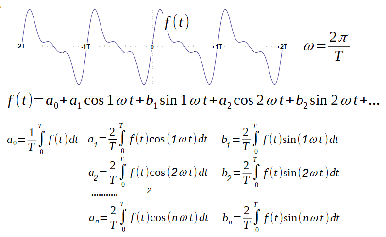

Fig. 2-1
Decomposition of the function f(t) on a Fourier Series where:
a0-constant component
1ω– pulsation of the first harmonic equal to the pulsation of the function f(t) here 1ω=1/sec.
2ω, 3ω… – pulsations of successive harmonics as multiples of the first
a1, a2 … – amplitudes of successive cosine harmonics
b1, b2 … – amplitudes of successive sine harmonics 
Parameters a0, a1, a2 …b1, b2 …an,bn calculated with the above integrals are specific values
E.g. for a odd square wave (Fig. 2-17)
a0=a1=a2=…=0
b2=b4=b6=…=0
b1=4/π=1.273, b3=4/3π, b5=4/5π…etc
For a this square wave, there are only odd coefficients bn in the figure. Even bn and all an are zero. So there are only sines. This is intuitive because sine and square wave are odd functions. If the graph were shifted π2 (90º) to the left, the square wave would be an even function and there would be only cosines.
Most often the Fourier Series is infinite, but not always.
Example of sum of sine waves:
f(t)=1.25sin(1t)+0.25sin(2t)
This series has only 2 coefficients b1=1.25 and b2=0.25. The others are zero.
The pulsation ω can be of any value. They are often ω=1/sec or ω=2π/sec, and then the Fourier Series has the following form: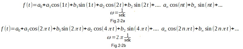

Fig. 2-2
Fig. 2-2a ω=1/sec slower waveform corresponding to period T=2π sec ≅6.28 sec
Fig. 2-2b ω=2π/sec faster run –> T=1 sec.

Chapter 2.2 Fourier Series Analysis – First Approach
I wonder what was on Jean Baptiste Joseph Fourier’s mind in 1806? How did he figure out that any periodical function f(t) is a sum of sine and cosine? I don’t know, but it could have been.
The trick is to find the appropriate coefficients ω,a0,a1,a2…b1,b2…of the equation f(t)=… from Fig. 2-1. Let’s approach the matter from the other side. i.e. we know the function f(t) and it is the sum of 3 sinusoids. To make it easier, there are no cosines! To draw it and then also to calculate it, we will use the amazing program from the Internet WolframAlpha. You don’t need to know him. Call only and enter in the appropriate fields what the picture below tells you. In this way, the function f(t) in the range t=-2π…+2π will be drawn. You will see how simple and useful this program is. I wrote more about the WolframAlfa program in the Rotating Fourier Series course in chapter 11.2. So click https:wolframalpha.com and do as the picture says. Anyway, you can be less ambitious and stop at just watching ready-made charts.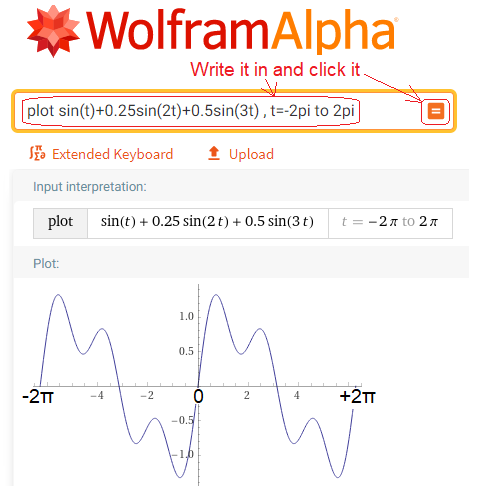

Fig. 2-3
The f(t) function was calculated and plotted with the command “plot”.
The domain of the function is t=- ∞…+ ∞ although the graph shows only t=-2π…+2π
It is a sum of sinusoids with pulsations and amplitudes:
First harmonic–> ω=1/sec (i.e. T=2π sec) with amplitude b1=1
Second harmonic–>2ω=2/sec with amplitude b2=0.25
Third harmonic–>3ω=3/sec with amplitude b3=0.5
The first harmonic corresponds to the pulsation ω=1/sec of our studied function f(t), i.e. the period T=2π sec.
The next ω pulsations are multiples of the first harmonic. Other parameters, i.e. b4,b5…a0, a1,a2..are zero. This is an example of a Fourier Series with a finite number of n=3 elements that I mentioned in Chapter 1.
Now imagine you only know the graph of f(t) but you don’t know the formula. All you know is that there are 3 sinusoidal components with unknown  ω1, ω2, ω3 pulsations and unknown b1, b2, b3 amplitudes .
As for the constant component a0, it is evident that a0=0. The fields “over” and “under f(t)” are the same!
The period T of the first harmonic ω1 should be the same as that of f(t), i.e. T=2π sec! After all, the first harmonic is the first approximation of this f(t) function. So ω1=ω=1/sec.
What is ω2 and ω3? They should be multiples of ω=1/sec, i.e. ω2=2/sec and ω3=3/sec. Otherwise, the harmonics would not meet at t=-2π, t=0, t=+2π… And they must meet for f(t)=0 at these points. Thanks to this, f(t) repeats every T=2π sec.
Now let’s move on to the other parameters, i.e. to the amplitudes of the b1, b2  b3  sine? Why not study their various combinations and choose such b1, b2 and b3 at which the sum of sine waves is closest to the f(t) function? After many, maybe even 100 attempts to draw the graph, we will get something closest to f(t) in Fig. 2-3. The combination will be, for example, b1=0.98, b2=0.2 and b3=0.48. Almost a success. These values are close to the formula. Let me remind you that we only know the graph f(t) but without the formula! A primitive, laborious and guesswork-like method. However, it is often used when the creative vema fails. It’s always better than waving a white flag.

Chapter 2.3 Fourier Series Analysis – Second approach with harmonic extraction
Mr. Fourier realized that the “guess-guess” in the previous chapter was only a prelude to solving the problem. How to cleverly extract individual 3 unknown harmonics? In fact, only 3 amplitudes b1, b2 and b3 because we already know the 1ω, 2ω and 3ω pulsations. And maybe so?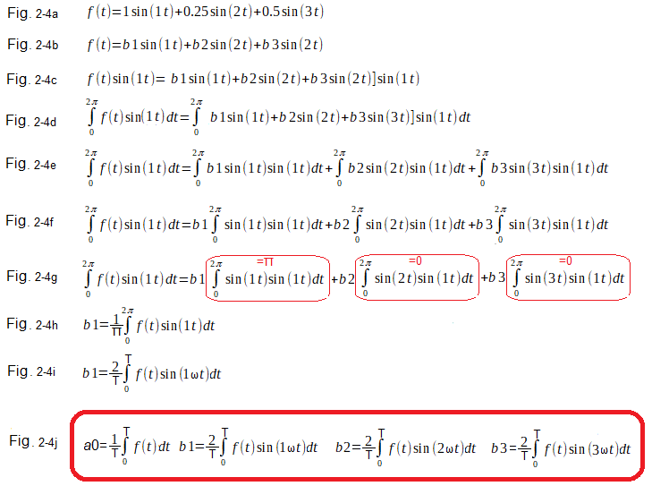

Fig. 2-4
How to extract the constant component, first, second and third harmonics?
Fig. 2-4a
Napoleon, who knew mathematics, asked Fourier*.
Dear Jean Baptiste – I thought of some function f(t) consisting of 3 sine waves.
What’s the function? For simplicity, I will say that its graph is Fig. 2-3 and its successive pulsations are 1ω=1/sec, 2ω=2/sec and 3ω=3/sec. I emphasize. You don’t know the formula of the f(t) function in Fig. 2-3, you only know its values in the range -2π…+2π, i.e. its graph.
Fig. 2-4b
Fourier wrote down this function with 3 unknown coefficients b1, b2 and b3 and started thinking.
First let’s find b1.
Fig. 2-4c
I’m looking for b1, so let’s multiply both sides of the equation by sin(1t)! Where did it come from? I guess he didn’t know himself. Probably intuition. Looking ahead, if you were looking for b2, for example, multiply by sin(2t).
Fig. 2-4d
Or maybe we could integrate both sides in the period T=2π. Where did Fourier’s idea come from? Probably intuition.
Fig. 2-4e
The integral broken down into sums.
Fig. 2-4f
Exclusion of b1, b2 and b3 before the integral.
Fig. 2-4g
And now the most important. Two integrals are zeroed and the first one is π!
Explanation in chapter 2.6.
Fig. 2-4h
Formula for b1 for pulsation ω=1, more precisely ω=1/sec. So for T=2π/ω=2π more precisely T=2πsec
Fig. 2-4i
Formula for b1 for arbitrary pulsation ω. So for T=2π/ω.
For ω=1, the formula transforms into Fig. 2-4h.
Fig. 2-4j
The final formula for a0, b1, b2 and b3 for f(t) from the plot in Fig. 2-3.
-a0 is the constant component f(t) which is the arithmetic mean. This is the mean of a function with period T.
-b1 is described in Fig. 2-4a…i
-b2 If in Fig. 2-4c we substitute sin(1t) for sin(2t), we get b2
-b3 If in Fig. 2-4c we substitute sin(1t) for sin(3t), we get b3
*Note
I don’t know if it was exactly like that, but the fact is that the gentlemen knew each other. Napoleon himself was even a good mathematician and is said to be the author of the theorem about the so-called Napoleon Points. Some, probably not fond of the chief, question it.

Chapter 2.4 Checking the formula
Chapter 2.4.1 Introduction
After applying the formula Fig. 2-4j for the function f(t) from Fig. 2-4a we get?
a0=0
b1=1
b2=0.25
b3=0.5
A bit like the riddle “The duck floats on the water, the duck’s name is”. After all, you can see it in Fig. 2-4a! Yes, but these coefficients are only for calculating the value of f(t)! Only to obtain, I hope, the correct coefficients from the integration formulas Fig. 2-4j. In other words, as if we had only f(t) graphs at our disposal.
Chapter 2.4.2 Constant component-a0
Enter the formula for a0 from Fig. 2-4j when T=2π to wolframAlpha.
Call up https://wolframalpha.com and do what the picture says.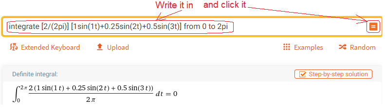

Fig. 2-5
Calculation of a0–constant component
As we expected a0=0. This can be seen in Fig. 2-3. The “areas above and below” are equal.
Chapter 2.4.3 First Harmonic Amplitude-b1
Call up https://wolframalpha.com and do what the picture says.

Fig. 2-6
Calculation of b1 – first harmonic amplitude
That’s right, b1=1, plus the integral is represented as an area
Chapter 2.4.4 Second Harmonic Amplitude-b2
Call up https://wolframalpha.com and do what the picture says.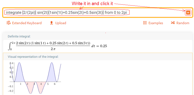

Fig. 2-7
Calculation of b2– second harmonic amplitude
That’s right, b2=0.25. Note that the “top” and “bottom” surfaces subtract.
Chapter 2.4.5 Third Harmonic Amplitude-b3
Call up https://wolframalpha.com and do what the picture says.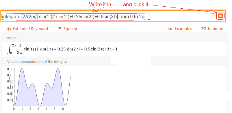

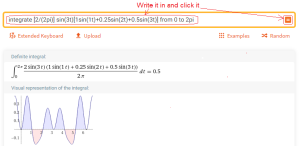
Fig. 2-8
Calculation of b3– third harmonic amplitude
That’s right, b3=0.5
Conclusions
Calculations from chapters 2.4.2…5 confirmed the truth of the formula Fig. 2-4j

Chapter 2.5 Orthogonal Functions
Chapter 2.5.1
Go back to Fig. 2-4g in Chapter 2.3 for a moment. There, two integrals were zero and one had the value of π. Now you will find out why?
Because in the zeros there were products of orthogonal functions, and in the one with π there were products of non-orthogonal functions.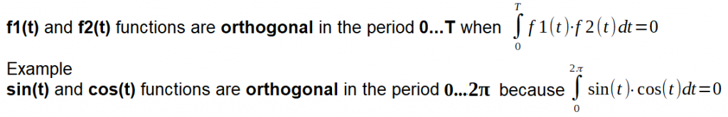

Fig. 2-9
Definition of orthogonal functions
For an electrician, the sinusoidal current and voltage across the coil are orthogonal functions because the energy in period T is zero! For one half of the period, the coil receives energy and for the other half it gives it back.
We will study the orthogonality of various combinations of pairs of sin(nωt) and cos(kωt) functions.
It turns out that:
Only the combinations sin(nt)*sin(nt) and cos(nt)*cos(nt) are not orthogonal and their integral=π
The other combinations sin(nt)*cos(kt) are orthogonal and their integral=0.
Chapter 2.5.2 Are sin(t) and cos(t) orthogonal?
The Fourier Series requires the ability to integrate. In order not to go too deep into mathematics, into some antiderivatives and other integration by parts, we will again use the wonderful program Wolframalpha From the integration itself, it is enough to know that the integral is defined by the area under the function.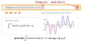
For example, we will check whether sin(t) and cos(t) are orthogonal.
Click https://wolframalpha.com and do as the picture says.

Fig. 2-10
How did WolframAlpha check the orthogonality of the functions f1(t)=sin(t) and f2(t)=cos(t)?
It couldn’t be simpler and more intuitive!
In the following sections, we will check the orthogonality of various combinations of sin(nωt) and cos(kωt).
You will find that the functions sin(nωt) and cos(kωt) are almost always orthogonal except for the pairs sin(nωt) and sin(nωt) or cos(nωt) and cos(nωt) whose integrals are T/2.
Chapter 2.5.3 The pairs sin(nωt) and cos(kωt) are orthogonal
Call https://wolframalpha.com and check orthogonality e.g. for ω=1, n=2 and k=3 i.e. for f1(t)=sin(2t) and f2(t)=cos(3t).
In the dialog box, instead of “sin t cos t” enter “sin 2t cos 3t”
Wolfram Allfa will calculate something like this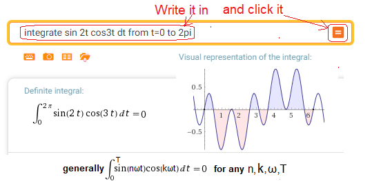

Fig. 2-11
The pairs sin(nω) and cos(kω) are always orthogonal. Also for n=k.
I leave the generalization to arbitrary pairs of sin(nωt) and cos(kωt) to mathematicians. This remark also applies to the next examined pairs of functions.
Note:
Although the periods of sin(2t)=2π/ω=2π/2=π and sin(3t)=2π/3 are different, the period of the product sin(2t)sin(3t) is equal to the period of sin(t), which is 2π ≈6.28. This can be seen in Fig. 2-11! Try to prove it.
In general, the period T of sin(nωt)*cos(kωt) is equal to the period sin(ωt) so T=2π/ω.
Chapter 2.5.4 The pairs sin(nωt) and sin(kωt) and cos(nωt) and cos(kωt) for n≠k are orthogonal.
I suggest you check the orthogonality of the function pairs sin(2t)sin(3t) and cos(2t)cos(3t) yourself with Wolfram Alpha.
Call https://wolframalpha.com
The result should be as follows: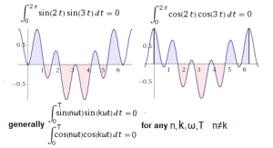

Fig.2-12
Orthogonality of pairs of functions sin(2t) and sin(3t) as well as cos(2t) and cos(3t) and their generalization.
Chapter 2.5.5 The pairs sin(nωt) and sin(nωt) and cos(nωt) and cos(nωt) are not orthogonal!!!
I suggest you check the orthogonality of the function pairs sin(2t)sin(2t) and cos(2t)cos(2t) yourself with WolframAlpha.
The result should be as follows: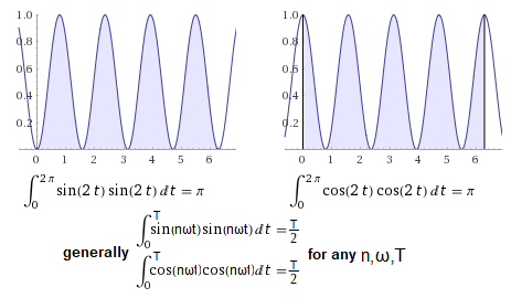

Fig.2-13
Orthogonality of pairs of functions sin(2t) and sin(2t) as well as cos(2t) and cos(2t) and their generalization.
The functions are not orthogonal and their integral = π for ω=1 and generally integral = T/2 (half period) for any ω pulsation.

Chapter 2.6 What are the parameters a0, a1, a2…an,,, b1,b2…bn Fourier series?
Chapter 2.6.1 Introduction
You’ll see in a moment how orthogonality makes it easier to find a Fourier Series. By the way. Orthogonal or perpendicular can be vectors, but functions? In Hilbert spaces they are supposedly the same as in our “human” spaces. Here the functions sin(ωt) and cos(ωt) are associated with rotating vectors with speed ω. The vector cos(ωt) leads the vector sin(ωt) by 90º and both vectors are perpendicular to each other. Otherwise, sin(ωt) and cos(ωt) are orthogonal.

Chapter 2.6.2 Coefficient a0
This is the average value of the function f(t) ie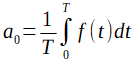

Fig. 2-14
Coefficient a0 as the average value of the function f(t) in period T
Chapter 2.6.3 Coefficient a2
This is a bit like chapter 2.3 on extracting harmonics Let’s calculate, for example, the coefficient a2.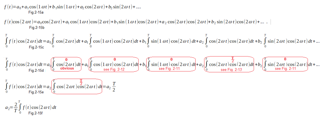

Fig. 2-15
How to calculate a2 coefficient?
Fig. 2-15a
Write the formula for the Fourier Series with the coefficients not yet known. We already know the coefficient a0.
Fig. 2-15b
Multiply both sides of the equation by cos(2ωt) because we are looking for a2
Fig. 2-15c
Calculate the definite integral of both sides of the equation in the range 0…T
Fig. 2-15d
The values ​​of the integrals have been calculated with reference to the relevant figures. The integral at a0 is zero, as with cosines.
Fig. 2-15e
After including the zeros in Fig. 2-15d
Fig. 2-15f
Final a2 formula

Chapter 2.7 Determination of the Fourier series formula
We have just determined the coefficient a2 of the Fourier Series. Similarly, we compute any an by multiplying both sides of the equation in Fig. 2-15b by cos(nωt) instead of cos(2ωt). However, if we multiply by sin(nωt) we get the coefficient bn. Taking into account the formula for a0 in Fig. 2-14, the final formula for the coefficients a0,an and bn of the Fourier Series is as follows: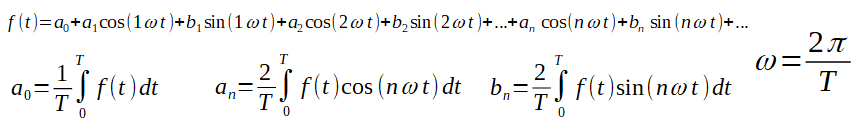

Fig. 2-16
Fourier Series formula
Note the pulsation ω of the periodic function f(t) and its relation to the period T.

Chapter 2.8 Determination of the Fourier Series for a Square Wave
Chapter2.8.1 Fourier series of a square wave directly from the formula
That is, for the time course presented in the time chart.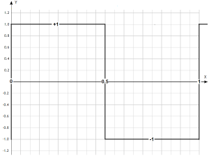

Fig 2-17
Square wave with period T=1 sec corresponding to pulsation ω=2π/sec
Let’s find a0, a1,a2,…a7 and b1,b2,…b7. Let’s use the general formula Fig. 2-16. We will use the Wolfram Alfa program to calculate the integrals. Fig. 2-18 is the result of calculating the coefficients a0, a1 and b1. I will admit to a slight correction-fraud. The program calculated a1 as an unimaginably small number, but still different from 0, and b1 as 1.27324, and not as mathematics says b1=4/π. I corrected this imperfection, also for the other coefficients.
Call https://wolframalpha.com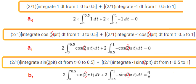

Fig. 2-18
Calculation of a0, a1 and b1 for a square wave Fourier Series from Fig. 2-17
The remaining coefficients a2, a3,a4,a5,a7 and b2,b3,b4,b5,b7 are also calculated with WolframAlfa. All you have to do is enter 4, 6, 8, 10, 12 and 14 in the dialog box, respectively, in the place of “2 in the red border”. The following table should appear.
Call https://wolframalpha.com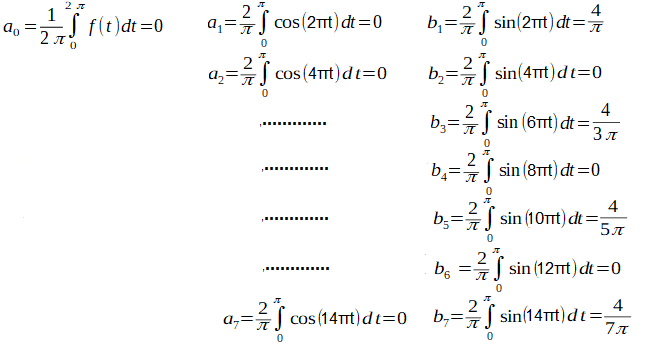

Fig. 2-19
Coefficients a0,a2, a3,a4,a5,a7 and b1,b2,b3,b4,b5,b7 of the Square Wave Fourier Series of Figure 2-17
By the way. The function is odd and therefore all coefficients a1, a2, a3… are zero. If it was even (e.g. shifted to the left by 0.25) then the coefficients b1, b2, b3… would be zero while a1, a2, a3… non-zero. This is intuitive.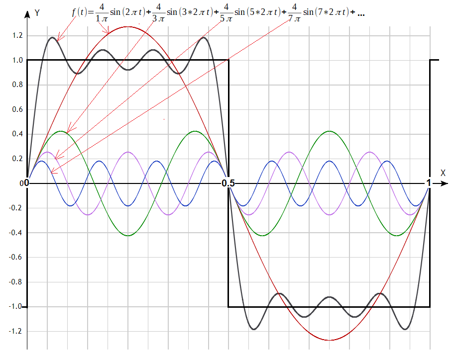

Fig. 2-20
Square wave decomposition into 4 harmonics.
Actually, the first 7, because b2=b4=b6=0. The pulsation of the first harmonic is ω=2π. The period T=1 corresponds to it. The more harmonics, the closer their sum is to a square wave.
Chapter 2.8.2 Fourier series of a square wave using the special functions of Wolfram Alfa
Previously, we determined the 7 harmonics of a square wave using the general integration instructions of the WolframAlfa program. The program also has specialized instructions for determining the Fourier Series. All you have to do is enter them into the dialog box and it will calculate it and make a graph! You don’t even need to know integrals.
Let’s check WolframAlfa for the same square wave. The effect should be identical.
Let’s not go into the details of the instruction typed into the dialog box. Let it suffice to know that it computes Fourier Series parameters for a square wave with the parameters of Fig. 2-17. It will count the first 7 harmonics. If you wanted to count them, e.g. 9, instead of 7, just enter 9.
Call https://wolframalpha.com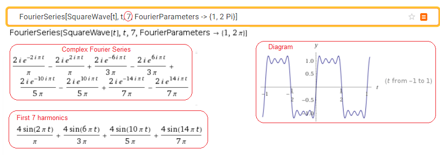

Fig. 2-21
Square wave distribution from Fig. 2-17 into 7 harmonics
The program will show us a lot of different things. Only the most important ones are shown in Fig. 2-21. The Complex Form of Fourier Series will be covered in Chapter 4. The important thing is that the graph and coefficients are exactly the same as in Fig. 2-20. And how much less work!
Then let’s check this miracle to determine the first 9 harmonics.
Call https://wolframalpha.com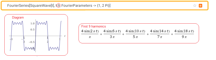

Fig. 2-22
Square wave distribution from Fig. 2-13 into 9 harmonics.
This is a more accurate approximation of a square wave.
Is it, for example, 17 harmonics? There should be an even more accurate approximation.
Call https://wolframalpha.com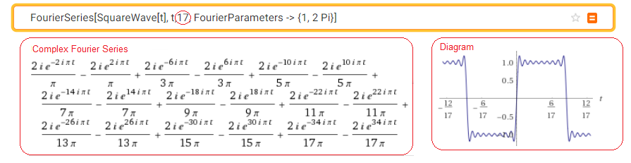

Fig. 2-23
Square wave distribution from Fig. 2-17 into 17 harmonics
The chart more accurately represents a square wave. Unfortunately, he did not give us the trigonometric version of the Fourier Series as before. This is not a major drawback, because the relevant parameters can be read from the complex form. When trying to determine 19 and more harmonics, the WolframAlfa program does not work anymore. I suspect it has some special gates though. Maybe the paid WolframAlfa Pro will do it?
The overshoot at the beginning of each pulse is called the Gibs effect. Appears when n has a finite value and disappears when n=∞.

Chapter 2.9 Determination of Fourier Series for other periodic functions
Chapter 2.9.1 Function 1sin(t)
I wonder how WolframAlfa will behave with such a trivial function?
Call https://wolframalpha.com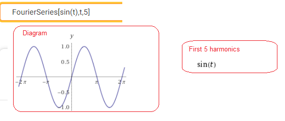

Fig. 2-24
Distribution of sin(t) into 5 harmonics.
The above instruction concerns the decomposition of the periodic function (here sin(t)) into 5 harmonics, with the additional assumption that T=2π, i.e. ω=1.
It is obvious that the first harmonic is the same function, i.e. sin(t) and the other harmonics do not exist, or otherwise their amplitudes are zero. The tacit assumption T=2π, i.e. ω=1 also applies to the following examples.
Chapter 2.9.2 “Ramp;” or function t
Call https://wolframalpha.com
Let me remind you that this is a periodic function with T=2π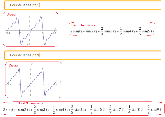

Fig. 2-25
The “Ramp” decomposition, i.e. the function t into the 5th and 9th harmonics.

Chapter 2.9.3 The quadratic function, the function t^2
Call https://wolframalpha.com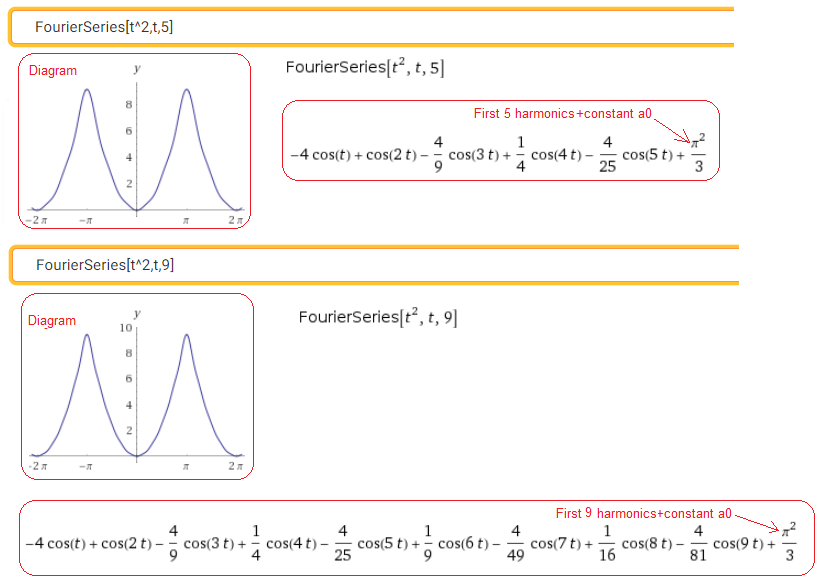

Fig. 2-26
Decomposition of a quadratic function into 5th and 9th harmonics. Note that in the range -π…+π, the 9-harmonic approximation visually does not differ from the quadratic function. By the way, we learned that there is such a thing as a constant component a0. It wasn’t there in the previous examples.