Automatics
Chapter 13. Differential Equations
Chapter 13.1 Introduction
This is the first approach to differential equations. We will analyze the process of filling the tank without a hole and with a hole in the bottom. Then simple differential equations will appear. There will be a lot of descriptions and the topic is not the easiest one. But try to face it. If there are still problems, raise the white flag and read on from chapter 14. Only then treat the transfer function G(s) as “something” that converts input x(t) to output y(t).
Chap. 13.2 Filling the tank without a hole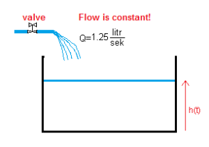
Fig. 13-1
Flow Q=1 liter/sec means that 1 liter of water flows out of the tap in 1 second.
Generally – Flow is the volume of liquid that flowed out of the tap in 1 second. At the same time, it is the volume of liquid V(t) by which the tank was enriched in 1 second. So we can easily calculate the volume V(t) after time t or the height h(t). But only if the flow is constant over time! So we do not turn the valve, as we have done many times with the slider.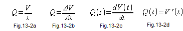
Fig. 13-2
Fig. 13-2a is the flow formula, provided that we do not turn the valve. So it’s constant. And when it’s not constant? Then the approximate formula for instantaneous flow appears (Fig. 13-2b), where ΔV is the volume of liquid in the tank that flowed out in time Δt. This formula is the more accurate the shorter the time Δt. Then the flow Q(t) becomes more and more similar to the derivatives shown in Fig. 13-2c or Fig. 13-2d. These are the simplest forms of differential equations.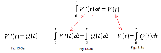
Fig. 13-3
Fig. 13-3a is a differential equation whose “known” is the flow function Q(t) and the unknown is the volume function V(t). We do not yet know what the V(t) time charte is, but we know that its derivative from V(t) is the Q(t) flow. How to find the V(t) function that satisfies this equation?
In the case when Q(t) is constant, as in Fig. 13-1 Q=1/liter/sec, the matter is trivial. V(t)=Q*t. A typical linear function. V(t=0)=0, V(t=1 sec)=1 liter, V(t=2 sec)=2 liters, etc.
And when Q(t) is time-varying? Then we solve the differential equation in Fig. 13-3a by integrating both sides.
Fig. 13-3b is the “integrated on both sides” equation Fig. 13-3a
Fig. 13-3c is the result of “bilateral integration”. Red arrows and Fig. 12-7c from chapter. 12 tell why.
By the way. Already in elementary school, in tasks like “A train goes from city A to B at a constant speed…” you were solving differential equations! The velocity V is the derivative of the distance S. When the velocity is constant, the formula S=V*t is a solution to the differential equation S'(t)=V. But let’s go back to the tank without a hole as an example of the simplest differential equation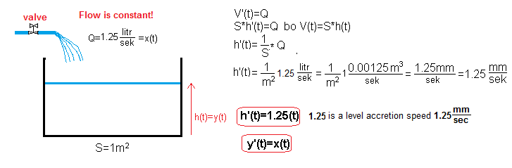
Fig. 13-4
The formula V'(t)=Q(t) is in other words “instantaneous flow Q(t) derivative of flow V(t)“, more figuratively – volume growth rate V'(t). When you fill the bathtub, the speed of increasing the volume V'(t) is more associated with the speed of increasing the level in the bathtub h'(t). Let’s try to simplify the general formula V'(t)=Q(t) as much as possible.
Assuming that:
– the bathtub is a rectangular prism with an area of 1 m²
– at the time t=0, we quickly turned on the tap and from then on there is a constant flow Q=1 liter/sec
– the bathtub is governed by the differential equation
h'(t)=1.25(t)
where 1.25(t) is the flow unit step from 0 to 1.25 liters/sec, and more generally y'(t)=x(t) where x(t) is the input and y(t) is the output.
Our goal is to find a h(t) function that satisfies this equation. Let’s integrate both sides of the equation as in Fig. 13-3c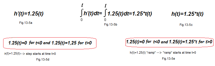
Fig. 13-5
Fig. 13-5a – differential equation describing the filled tank, where the output is the water level h(t)
Fig. 13-5b – integration of both sides of the version from Fig. 13-5a
Fig. 13-5c-solution as a result of the above integration
Fig. 13-5d – definition of the flow step 1.25(t) as the input signal
Fig. 13-5d – definition of the solution as an increasing sawtooth of the level h(t)
Let’s solve the differential Fig.13-5a equation using the free Scilab program.
Fig. 13-6
From chapter 12, e.g. Fig. 12-14, we know that the output of the integral unit is the integral of the input and vice versa, the input is the derivative of the output. Therefore, we conclude that x(t)=y'(t), i.e. 1.25(t)=h'(t). Thus, the scheme in Fig. 13-6 solves the differential equation h'(t)=1.25(t). Let’s check it:
At the moment t=0, the valve opened immediately. From now on, the flow Q(t)=1.25 liter/sec is constant. The time chart shows that the water level rises at a constant speed in accordance with the formula h(t)=1.25*t(t), where the level is given in millimeters. e.g. In 10 seconds, the water level in the tank is h=12.5 mm.* Let me remind you that for t<0 (negative) x(t)=y(t)=0.
*Don’t worry about the strange size of the tank in which S=1m2 and the level h(t) will rise by approx. 12.5mm.
Chapter 13.3 Filling a tank with a hole k=1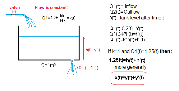
Fig. 13-7
Unlike Fig. 13-4, the water level will rise more and more slowly due to the outflow of Q2(t). Previously, the rate of level rise h'(t) was proportional to the input flow Q(t), so now it will be proportional to the flow difference Q1(t)-Q2(t). We know that the higher the water level, the greater the outflow. So Q2(t)=k*h(t). Question. How k depends on the area of the hole? Sure, the bigger the hole, the bigger k! When k=0, there is no hole and there is the previous case, i.e. Fig. 13-4.
Let’s assume that the size of the hole corresponds to k=1.
The figure shows that the above tank is described by the differential equation:
1.25(t) = h'(t) + h(t)
and more generally:
x(t)=y'(t)+y(t)
Let’s try to predict which h(t) function satisfies this equation? I can’t seem to get on my fingers anymore. Integrating the two sides of the equation, as for the equation x'(t)=y(t), will not help either. There are methods, of course, but we don’t know them yet. Maybe we can at least partially predict how the h(t) level behaves over time?
Certainly for t=0 h(t)=0. Then 1.25=h'(t). Slope (derivative!) of the h(t)=1.25. In a moment h(t) is no longer zero and h'(t)=1.25(t)-h(t) . The slope h(t) will decrease a bit. The level is rising a little slower, and the outflow of Q2(t) will increase a bit. And when will the level settle? Then when what goes in, goes out. That is, when Q2(t) = Q1(t). When the level is fixed, h'(t)=0 and h(t)=1.25 mm. Doesn’t this remind us of the inertial unit?
Let’s solve the differential equation using a diagram with an integrating unit. So we will use the Xcos application of the free SCILAB program.
Fig. 13-8
For each integral term 1/s, its input is the derivative of the output. And it doesn’t matter if the input is a single signal as in Fig. 13-6 or a difference of 2 signals as in Fig. 13-8. It can even be any function of several signals, e.g. a product. Therefore, the integrating unit is ideal for solving such differential equations where y(t) and its derivative y'(t) occur.
So h'(t)=1.25(t)-h(t) otherwise 1.25(t)=h'(t)+h(t) and generally x(t)=y'(t)+y(t)
The scheme will give y(t) where the equation x(t)=y(t)+y'(t) is satisfied at any time.
It seems that the tank with the hole is an inertial unit. The graph shows that the time constant T=1 sec. After 6…7 seconds, the tank will reach a constant level h=1.25 mm.
Notice that the equation 1.25(t)=h'(t)+h(t) holds true all the time. At the beginning, the derivative h'(t) is the largest and equals 1.25 mm/sec and the level h(0)=0. Then the slope decreases and the level increases. In steady state, the slope, i.e. h'(t)=0 and h(t)=1.25.
A little comment.
After approx. 7 sec. the water level was set at h=1.25 mm. Very small this level, there is only 1.25mm at the bottom! Apparently the hole is so big that the bottom will only become wet. Let’s double the area of the hole. So let’s say k=0.5. Will the level be twice as large?
Chapter 13.4 Filling a tank with a smaller hole k=0.5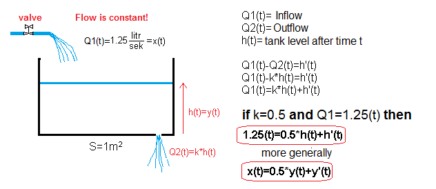
Fig. 13-9
Now the hole is smaller (k=0.5) and the bath is described by the differential equation:
1.25(t)=h'(t)+0.5*h(t)
and more generally:
x(t)=y'(t)+0.5*y(t)
Compare with the previous tank and find the difference.
We will solve the differential equation using a scheme with an integrating unit
Fig. 13-10
As we expected, the fixed level will be 2 times higher. Here y=2.5 mm. As for the dynamics, the system is still inertial but has a time constant twice as large ->T=2 sec.
Note
We assumed that the water outflow is proportional to the level Q2(t) = k*h(t). Indeed, when I pull out the plug in the bathtub, the water flows the fastest at the beginning, then (when the level is lower) it flows slower! However, this is only a first approximation! In fact, the Q2(t) outflow is proportional to the root of the level! So let’s check out this more accurate mathematical model.
Chapter 13.5 Filling the tank with a hole k=1-more accurate model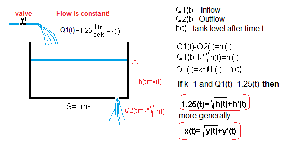
Fig. 13-11
The above equations show that the Q2 outflow is proportional to the root of h(t). The resulting equation is an example of a non-linear differential equation, usually more difficult to solve than the previously considered linear ones. Fortunately for Xcos, this is no problem.
Fig. 13-12
At first glance, it looks like an inertial unit. But he is not! Compared to chapter 13.3, where k=1 was also present, the liquid reached a higher fixed level h=1.5625 mm. This level can also be determined theoretically. Then the inflow of Q1(t) is equal to the outflow of Q2(t).
One more thing. Remember that I assumed a step x(t)=1.25(t) instead of x(t)=1(t) as usual. Why? Because for x(t)=1(t) the levels determined for the tank “with a hole” and “without” are exceptionally the same h=1mm! . The reader might think that this is the case for any x(t).
Chapter 13.6 More on differential equations
In a tank without a hole, we learned the simplest differential equation 1.25(t)=h'(t)
A tank with a hole is described by a more difficult differential equation 1.25(t)= h'(t)+h(t)
The last equation can be generalized to x(t) = a1*y'(t) + a0*y(t) where:
– x(t) – input signal – equivalent to step 1.25(t)
– y'(t) – derivative of the output signal – equivalent of h'(t)
– y(t) – output signal – equivalent of h(t)
– a0, a1 constant coefficients – in equation 1.25(t) = h'(t) + h(t)–> a1=a0=1
The equation can be further generalized to a higher degree of derivative – e.g. degree 3.
– x(t) = a3*y”‘(t) + a2*y”(t) +a1*y'(t) +a0*y(t)
a0, a1, a2, a3 are constant coefficients.
Since we’re generalizing so well, the derivatives can also be on the left-hand side, e.g.
– b3*x”'(t) + b2*x”(t) + b1*x'(t) + b0*x(t)= a3*y”'(t) + a2*y”(t) + a1*y'(t) + a0*y(t)
An example of a non-linear differential equation was a more accurate model of a tank with a hole from Chapter 13.5 or, for example,
y(t)*x”(t) + t*x(t) = y(t)”+x(t)*y'(t) + y(t)
We will not deal with such equations. Therefore, each differential equation will be a linear differential equation for us.
And how to solve them? So how to find the function y(t) knowing the function x(t)? Turns out you’ve done it many times in this course. The input signal x(t) was most often a unit step 1(t), less often a linear or quadratic signal.
Then Xcos based on:
– block diagram
– input signal x(t)
created the appropriate linear differential equation, which he solved by calculating y(t) and showed on the time chart. It is known that differential equations can also be solved on paper. Mathematicians have been doing it for a long time, before there were computers and Xcos.
In the next chapter, we will deal with operatotional calculus as a tool for solving linear differential equations.