Automatics

Chapter 7 Oscillation Unit
Chapter 7.1 Introduction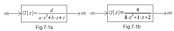

Fig. 7-1
The oscillatory unit and the previously known two-inertial unit are examples of transmittance G(s) in which the numerator is a constant number d, and the denominator is a binomial of the second order with parameters a, b, c–>Fig. 7-1a.
In Fig. 7-1b parameters a,b,c,d have specific values 8,1,2,4.
From the general form, Fig. 7-1, it is not clear whether it is a two-inertial or oscillatory unit.
Therefore, G(s)–>Fig7-1a should be transformed into a normalized form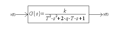
Fig. 7-2
Oscillatory Unit-Normalized form
And in it:
k – steady state reinforcement
q – damping factor – the higher it is, the stronger the oscillation damping
T – coefficient of the oscillation period. I only emphasize. Factor T, not the oscillation period itself Tosc.
The theoretical period of oscillation will be calculated according to the formula Tosc=2*π*T. Moreover, it is an approximate model. The true oscillation period on the diagram will be accurate only for damping q=0. Damping q increases this Tosc period.
Normalized G(s) is a bit bizarre, but everything will be clear after examining the specific transmittance G(s) from Fig. 7-1b.
To begin with, let’s bring it to a normalized form, i.e. as shown in Fig. 7-2.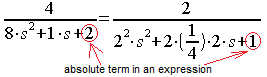

Fig. 7-3
And how to do it?
1 Divide the numerator and denominator by 2, so that the free component of the expession (i.e. without s) becomes 1
2 … etc
Of course L=P and check it out.
In this way, we will get the normalized form on the right. It shows that k=2, T=2 sec (i.e. Tosc=2*π*T=12.56 sec) and q=0.25. In the next sections, we will study this transmittance and its modifications at various attenuations q.
Note
The value of the damping coefficient q results in:
q=0–> ideal oscillating unit – no damping –>Chapter. 7.5
0<q<1 real oscillating unit– with damping–>Chapter. 7.2 , 7.3 , 7.4 , 7.6
q>=1 two-inertial unit–>Chapter. 7.7
It’s lab time!

Chapter 7.2 k=2 T=2 sec q=0.25 with slider and bargraph
We start with the slider and the bargraph. It is true that it is difficult to read the oscillation parameters by observing the bar graph, but you will feel the weight on the spring. It will come in handy in the pub brawl.

Fig. 7-4
x(t)=0.5
You will see oscillations. Wait a bit until it calms down and calculate the gain k using steady-state digital meters. It should be k=2. With the parameters T and q let’s leave it alone for now. We’ll come back to them using an oscilloscope.

Chapter 7.3 k=2 T=2 sec q=0.25 with step and oscilloscope
What will be the real oscillation period Tosc from the graph compared to the theoretical Tosc=12.56 sec calculated in Fig. 7-3?

Fig. 7-5
Gain k=2 agrees perfectly with the theory.
The real period of the oscillation Tosc=13 sec on the oscilloscope is slightly larger than the
theoretical Tosc=12.56 sec*. And the damping q? You can also calculate this parameter from the graph, but let’s spare it. It is enough for us to know that q increases Tosc and causes faster decay of vibrations. We will see this in the next experiments.
*Tosc=2*Π*T=12.56 sec

Chapter 7.4 k=2 T=2 sec q=0.125 with step and oscilloscope
How will reducing the damping twice to q=0.125 affect the waveforms?

Fig. 7-6
Oscillations last longer. and they didn’t even have time to calm down until 60 seconds. The oscillation period has decreased to Tosc=12.9 sec but is still greater than ideal Tosc=12.56 sec.
Gain k=2 is obvious. The first amplitude also increased.
What if we could completely get rid of damping by giving q=0?

Chapter 7.5 Ideal Oscillatory Unit k=2 T=2 sec q=0 with step and oscilloscope
How will the lack of damping, i.e. q=0, affect the waveforms?

Fig. 7-7
What’s up? There is no steady state y(t)=2. Instead, there is a constant component 2 around which a sine wave with an amplitude also 2 “flies”. And it will be like this until the end of the world. Notice that the real Tosc=12.56 sec from the graph is equal to the theoretical one. This is a feature of an Ideal Oscillating Unit.
So far, we have been reducing the damping until we have reached the ideal oscillatory where q=0. Now let’s go the other way with damping and increase it to q=0.5.

Chapter 7.6 k=2 T=2 sec q=0.5 with step and oscilloscope

Fig. 7-8
The output y(t) seems to approach a two-inertial one, although it is still an oscillatory unit. The amplitude decreased and Tosc=14.8 sec increased. The most deviates from the theoretical 12.56 seconds now. So let’s go all out and give q>1, e.g. q=1.5.

Chapter 7.7 “Oscillating”unit k=2 T=2 sec q=1.5 with step and oscilloscope
The name “Oscillating” in quotes and double-inertial in the title suggest something. It’ll clear up in a moment.

Fig. 7-9
Exactly. Typical response of the two-inertial unit. It turns out that for q>1 the oscillatory unit becomes two-inertial!. Hence the quotation marks in the title of chapter 7.7. Since it is two-inertial, the transfer function from Fig. 7-9 can be reduced to the form from Fig. 6-1 from the previous chapter 6.

Chapter 7.8 “Oscillating” unit k=2 T=2 sec q=0.25 with Dirac and oscilloscope

Fig. 7-10
Dirac shows what is most interesting in the oscillatory unit – only a variable component.
Tosc=13 sec is the same as in Fig. 7-5.

Chapter 7-9 Four with dirac and oscilloscope simultaneously
As a summary, we will give a simultaneous dirac pulse to 4 dynamic units with different damping q. They all have T=0.5 sec and k=1 We chose dirac as x(t). Then the response does not have a constant component and it is easier to observe the effect of damping q on the time waveforms.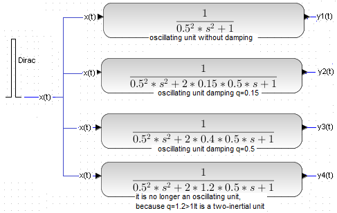

Fig. 7-11
The same short but strong signal x(t) is fed to the inputs of successive terms with a decreasing damping factor q.
This short x(t) “hammer blow” is an approximation of the ideal Dirac pulse..

Fig. 7-12
There is a clear influence of q damping. The greater the damping, the less the tendency to oscillate.
For the largest q=1.2, there is no longer even an oscillating unit but two-inertial unit

Chapter 7.10 Conclusions
1. The transmittance of the oscillating unit for 0 <q<1 is shown in Fig. 7-2.
2. For q=0 it is an ideal oscillating unit in which the vibrations never die out.
3. With increasing damping q the oscillations decrease. The oscillation period Tosc also increases.
4. For q>=1 we are dealing with a two-inertial ubit. Then the denominator G(s) can be presented as in Fig. 6-1 in chapter 6

The transmittance of the oscillating and two-inertial units can also be said differently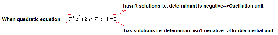

Fig. 7-13
The same can be expressed using complex numbers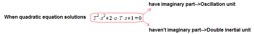

Fig. 7-14
Knowledge of complex numbers is not necessary, but if you want something more, click Courses in the header and select the Complex Numbers course.