Automatics
Chapter. 6 Double Inertial Unit
Chapter 6.1 Introduction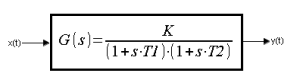
Fig. 6-1
Transmittance of the Two-inertial unit with gain K and time constants T1 and T2
Previously, an example of an Inertial Unit was a furnace. At the beginning, the temperature increases the fastest, then the temperature speed gradually decreases (but the temperature itself continues to increase!). Eventually it will stop growing and reach a steady-maximum state, e.g. +150 °C. At the beginning, the temperature rises the fastest? Is it? If you look closely, nothing happens at first. That is, the initial rate of temperature increase is zero. Only then the temperature gradually accelerates and at some point the speed reaches its maximum. (Velocity that is a derivative of temperature, not the temperature itself!). From that moment, the speed decreases until it becomes zero and the temperature reaches a steady-maximum value.
So the Inertial Unit as a furnace model is only its first approximation. The Two Inertial Unit is more accurate. But not overly accurate, because as you will see in a moment, the initial speed, although not maximum, is not zero either.
Chapter 6.2 Slider as input and bar graph as output
Fig. 6-2
A Two Inertial Unit as a serial connection of two Inertial ones.
yp(t)-indirect signal from the first inertial unit.
“Waving” the slider and observing the bar graph is only a preliminary familiarization with the object. You may notice a gradual “acceleration” of the temperature. But you’ll definitely notice a feature of the Two-Inertial that the Inertial didn’t have.
The +maximum slider input is given, and when y(t) is the most accelerated, –minimum is given. You will surely notice that the output signal continues to grow, although the input is not only zero but even negative!
This is also true in a real oven. The temperature continues to rise even when the power supply is interrupted.
When observing digital meters, you will notice that the intermediate signal yp(t) “leads” the output signal y(t).
You will notice more interesting things, including the inflection point, by examining the waveforms on the oscilloscope.
Chapter 6.3 Input signal x(t) as a unit step
Fig. 6-3
The “transition” signal yp(t) behind the first inertia clearly precedes the second inertia y(t) – i.e. the output of the Double-Inertial unit. The acceleration effect is also visible. Around second 6, the rate of increase of y(t) (i.e., the derivative y'(t)) is the highest. Here is the so-called inflection point of the function y(t) After 29 seconds we have a steady state y(t)=1. Then the velocity y(t), i.e. the derivative y'(t), is zero.
Chapter 6.4 Input signal x(t) as a single square pulse
Fig. 6-4
At time 8…8.7 sec, the output signal y(t) increases even though the input signal x(t) has fallen to zero! At this time, yp(t)>y(t) and this is what causes this phenomenon.
Ch.apter 6.5 Multi-Inertial units
Look at Fig.6-1. The denominator has two factors and is a two-inertial unit. If it had three factors, it would be three-inertial. And if there were many factors, it would be multi-inertial. The larger this “many”, the slower the initial velocity of the output signal y(t). Many processes in industry, especially chemical ones, are multi-inertial elements. In chapter 9 you will learn that they are approximated by the so-called substitute transmittance.