Automatics
Chapter 5 Differentiating Unit
Chapter 5.1 Introduction
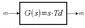
Fig. 5-1
Differential Unit transfer function G(s). More strictly – Ideal Differential Unit.
The Differential Unit reacts to the rate of change of the signal x(t), not to its value! It is the best teaching aid to understand the concept of the derivative of a function, in general calculus. Usually in transfer functions G(s), the letter s appears in the denominator of the fraction, while in the derivative unit it is an ordinary number (but complex s like any other in this article) in the numerator. (here denominator=1)
With manual control from the slider, the output waveforms of the derivative element are just mean, some pins, etc … This makes it difficult to draw the right conclusions. Therefore, when examining this unit, there will be no diagrams with a slider and a bargraph.
The Differential Unit component gives the output signal y(t) proportional to the rate of change of the input signal x(t), i.e. to its derivative.
Therefore, in each experiment, make sure that this is the case, i.e.:
When x(t) is growing rapidly–>y(t) is large positive
When x(t) is constant –> y(t)=0 because the velocity is zero
When x(t) is rapidly decreasing–>y(t) is large negative (negative speed)
Chapter 5.2 Signal x(t) increases linearly when Td=1sec
Fig. 5-2
The drawing is at first the same as for the integratitng unit in Fig. 4-4 in chapter 4 . But there was a step at the input and a ramp at the output, and here it’s the other way around! That is why it is said that differentiation is the inverse of integration and vice versa.
The most important
For the differentiator with transmittance G(s)=s*Td when Td=1sec, the y(t) output signal is equal to the rate of change of the x(t) input signal. The speed of change is 1/second and is constant. Therefore, the response to this signal is a constant value of 1.
The rate of change of any function is the derivative of this function. Here the derivative was easy to calculate, because the rate of change was constant.
The derivative of x(t) is y(t). Up to the third second, y(t)=dx/dt=0, because x(t)=0, and does not change, and from the third second, dx/dt=1.
Definition of differentiation time Td
After the time Td=1sec, the differentiator signal y(t) equals the increasing input signal x(t). Note that Td does not depend on the rate of increase x(t). When the speed increases, the alignment will also occur after Td=1sec, but at a higher level of y(t)!
Let’s repeat the experiment, but with twice the slew rate of the linear signal.
Fig. 5-3
A double increase in the growth rate of x(t) resulted in a double increase in y(t).
But equating x(t) with y(t) also happened after 1 second. The differentiating unit G(s)=s*Td is like a speedometer of the x(t) signal.
Chapter 5.3 Signal x(t) “rising, standing and falling”
A phenomenon known not only in automatics.
Fig. 5-4
0…2 sec constant x(t)=0 therefore y(t)=0 (because “speed” x(t)=zero)
2…4 sec signal x(t) increases with a constant (positive) rate=1/sec (derivative!)–> y(t)=+1
4…6 sec the signal x(t)=1 is constant, i.e. it has velocity=0 –>y(t)=0
6…10 sec the signal x(t) decreases with a constant (negative) speed =-1/sec –> y(t)=-1
Chapter 5.4 Signal x(t) with two constant speeds
Fig. 5-5
Doubling the speed (derivative) of the input signal x(t) resulted in a doubling of the output signal y(t).
Chapter 5.5 Signal x(t) with four constant speeds
Each time the speed, i.e. the derivative of the input signal x(t) will increase by the same speed increase Δx(t)=1/sek.
Fig. 5-6
A fourfold increase in the speed (derivative) of the input signal x(t) resulted in a fourfold increase in the output signal y(t).
The x(t) signal becomes similar to a parabola (square function) and y(t) to a linear one. Roughly, of course. What if you gave x(t) as a parabola as input? Can you guess what will happen?
Chapter 5-7 Signal x(t) is a square function
And if there are 8, 16, ….. 1024 … infinitely many of these segments, will we get a perfect parabola?
Let’s check.
Fig. 5-7
The Differentiating Unit confirms the formula for the derivative of a quadratic function known since the 17th century. Check, for example, that the derivative formula is valid for t=4.
Chapter 5.7 x(t) is the sine wave of sin(t)
Fig. 5-8
x(t)=sin(t) y(t)=cos(t)
The sine signal x(t)=sin(t) was differentiated by G(s) giving a cosine output.
A cosine wave is a derivative of a sine wave.
Chap. 5.9 x(t) is a single rectangular pulse
Fig. 5-9
In 3 seconds, the input signal x(t) increases as a step. So its growth rate has the value +infinity.
Hence this red pin y(t) is dirac to +infinity. In 6 seconds, the signal decreases to zero –>negative speed -> red pin y(t) is dirac to -infinity. In the rest of the time (i.e. everywhere except 3 and 6 seconds) x(t) is constant. So x(t) has zero velocity. So at this time y(t) is also zero.
Chapter 5.10 Conclusion
Differentiating Unit reacts to the rate of change of the input signal x(t), i.e. to its derivative x'(t).

Fig. 5-10
An example is a coil with inductance L, when the input x(t) is the current i(t) and the output y(t) is the voltage on the coil u(t).
A typical input signal x(t) for testing most dynamic units is a unit step. For the differentiating unit, however, it is a linearly increasing signal. Then it is easy to obtain the Td parameter from Fig. 5-1.
For a unit step ->Fig.5-10, it would be more difficult. Therefore, increasing signals x(t) of the sawtooth type are best suited for the study of differentiators.