Automatics
Chapter 4 Integrating Unit
Chapter 4.1 Introduction
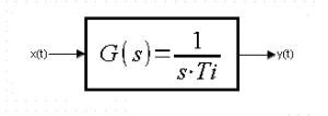
Fig. 4-1
Transmittance of the Integral unit
It is recommended when the transmittance numerator has a value of 1. Then the parameter – integration time Ti has an easy interpretation -> p.4.4. And when not? E.g. G(s)=3/9s? Divide the numerator and denominator by 3 and you get the same G(s)=1/3s, just in normalized form. Here you can see that Ti=3sec.
Note for those unfamiliar with integrals and derivatives.
Don’t worry for now. It is enough for you to associate the output signal y(t) with the input signal x(t) (usually a unit step) and the integration time Ti. Chapters 11 and 12 will be devoted to differentiation and integration
Chap. 4.2 Scheme with slider and bar graph
As usual, we start the description of the new dynamic unit with the slider and the bar graph. The response to the slider is more visual than math.
Fig. 4-2.
Observe the slider x(t) and bargraf y(t)
The input signal x(t) is a slider and a digital meter
The output signal y(t) is a bar graph and a digital meter
A typical feature of the integral unit is the speed of the output signal y(t) which is proportional to the input signal x(t).
You will find that:
– increased positive signal x(t) causes a rapid y(t) increase
– increased negative signal y(t) causes a rapid y(t) decrease
-zero signal x(t) stops y(t)
Note:
I had a problem setting x(t)=0, that’s why you see “almost x(t)=0” on the gauge.
That’s why it’s “almost stop” then
What does that remind you of? You have such a device at home. It’s a TV remote.
Once you enter the “plus” value ->the volume increases.
You will enter “zero” -> constant volume.
You enter “minus” -> the volume decreases.
Chapter 4.3 Scheme with slider and oscilloscope
And now x(t) input from the slider but y(t) output from the oscilloscope.
Fig. 4-3
I changed the x(t) signal with the slider. This can be seen in the x(t) gauge and the x(t) graph. The time plot clearly shows that the rate of change of the output y(t) is proportional to the input x(t). For example, when x(t) doubled around 13 second, the signal speed y(t) also doubled. Also x(t)=0 kept y(t) constant.
Chapter 4.4 Scheme with unit step x(t)=0.1 and oscilloscope
Chapter. 4.4.1 Ti=1sek
Fig. 4-4
The previous scheme, when the x(t) input signal came from the slider, allowed for the initial analysis of the integrator. Therefore, we will replace the slider with a more accurate unit step generator. More precisely, it will be a step x(t)=0.1.
Let’s repeat the experiment for Ti=2 sec.
Chapter. 4.4.2 Ti=2sek
Fig. 4-5
As expected, the signal will grow 2 times slower. The alignment took place after time t=Ti=2 sec. Now we can define the integration time Ti for the integral term from Fig. 1-1. This is the time Ti, after which the output y(t) equals the step input x(t).
Chapter 4.5 Scheme “with stairs” and an oscilloscope
Chapter 4.5.1 “2 stairs” and an oscilloscope
Fig. 4-6
Response to x(t) “2 stairs”
When the input signal increased 2 times, the speed of the output signal also increased 2 times.
Chapter 4.5.2 “4 stairs” and an oscilloscope
Fig. 4-7
Response to x(t) “4 steps”
With each step, the speed increases
Chapter 4.6 Scheme with a x(t) ramp-up signal and an oscilloscope
It is no coincidence that the previous input signals x(t) were stepped. Why? Because a linearly increasing signal can be treated as with an infinite number of small steps.
Fig. 4-8
When the input signal increases linearly x(t)=t then y(t) increases as a square function. Check by substituting different values for t.
The integrating unit, as the name suggests, integrates the input signal x(t) giving the output a parabola y(t).
On the other hand,calculus says that the definite integral of the function x(t)=t is also a parabola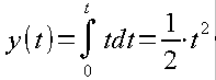
Fig. 4-9
Check that e.g. for t=4 x(t)=5, y(t)=12.5
Indeed, put t=5 and you will see. So theory matches practice. If you don’t know math, don’t worry. For now, consider that the definite integral from 0 to t of x(t) is the signal y(t) of the 1/s integrating unit.
Chapter 4.7 Scheme with positive and negative step and oscilloscope
This is better version of the experiment in Fig. 4-3, in which the x(t) signal is supplied from the generator, which is a more precise device than the slider.
Fig. 4-10
In a similar way, you control the volume on the TV with the remote control, but here you can also control the speed of the bar. It can also be an actuator as a DC motor with a gear. The input is the voltage and the output is the position of the actuator lever.
Chap. 4.8 Scheme with a Dirac pulse and an oscilloscope
Fig. 4-11
There is no perfect Dirac impulse in nature. There is only an approximation of it. Here, a rectangular pulse with an amplitude of 100 and a duration of 0.01 sec.
Chapter 4.9 Typical integrating units.
Capacitor.
Input – capacitor charging current
Output – voltage on the capacitor
When a capacitor is charged with a constant current, the voltage increases linearly, the faster the smaller the capacitance C of the capacitor
The bathtub is clogged with a cork.
I assume the bathtub is a rectangular prism.
Input – water flow from the tap, indirectly the degree of opening of the tap
Exit – water level
If the flow is constant, the water level will increase linearly. The faster the smaller the surface of the bathtub.
Electric actuator.
I assume we have an ideal dc gear motor.
Input – motor voltage
Output – position angle of the actuator shaft
A constant voltage on the motor will cause the angle to increase linearly. The rate of increase is proportional to the voltage.