Automatics

Chapter 30 Control Systems Structures
Chapter 30.1 Introduction
The structures do not depend on the type of controller. It can be PID, two-position and any other, e.g. discontinuous PID variants. Here a small digression to “discontinuous PID variants”. You read the specification of the two-position controller, and there is, for example, the Kp=3 setting typical for a proportional controller. What is it about? After all, he only turns the power on and off to the object. What Kp gain can a two-position controller have? But if it outputs a 1 Hz square wave with a duty cycle proportional to the error e(t), and the object has an inertia of the order of minutes, then we are dealing with almost continuous control! Thus, we have a two-position controller, which acts as a proportional one. Nay. There can be two-position PID controllers with Kp, Ti, D settings. The most typical representative of discontinuous PIDs is the so-called step controllers. It is most commonly used in flow control and is used to control the degree of valve opening. Here, the controller reaches the setpoint x(t) value by acting on the actuator with a voltage signal, e.g. +max, 0, -max in jumps, otherwise – in steps (increase, stop, decrease). All in all, although the control signal is discontinuous, due to the large inertia of the object, its response is continuous.
But let’s get back to the topic.
We will examine typical structures of control systems:
1– Opened loop
2– Opened loop with the noise compensation
3– Closed loop
4– Closed loop with the noise compensation
5– Cascade control
6– Ratio control

Chapter 30.2 Opened loop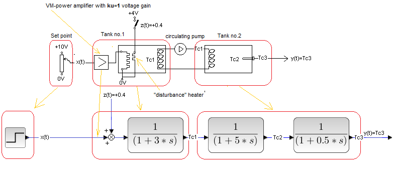

Fig. 30-1
An example is the heat exchanger control diagram above. It is convenient for the analysis when the actuator is part of the exchanger – the Go(s) object. Here the actuator is a power amplifier with a heater. An open system has some advantages- simplicity and it is always stable. On the other hand, it is completely vulnerable to disturbances z(t). The disturbance z(t)=+0.4 is a voltage spike of +4V caused by a short-circuit of the contact on the “disturbance” heater.
Every serious controller has an A/M switch for Auto/Manual operation.
Automatic operation A is the version Fig. 29-7 from chapter 29.
Manual work M is an open system, which is the figure above.
Then in Fig. 29-7 from chapter 29 the negative input to the controller has been connected to 0V, and the PID controller itself will change its P controller structure by Kp=1. In other words, the feedback loop was broken and an open system was created, i.e. Fig. 30-1.
Manual work is used during the commissioning of the facility, in emergency and other unusual situations.
The A/M switch can be a regular switch or just a software one. Then the operator switches A/M from the keyboard. Provides a smooth transition from mode  M and vice versa. It is somehow implemented there, but I will not go into details.
What will happen if we move the adjuster slider from 0 V to +10V in 3 seconds, and we give a +4V step to the “disturbance” heater in 40 seconds?
Note
Most controllers are implemented in a digital version. In other words, addition, subtraction, multiplication, division, integration and differentiation are calculated by the microprocessor, not analog.

Fig. 30-2
It’s like you suddenly moved the slider from 0V to +10V, and then in 40 seconds gave a step of +4V to the disturbance heater. The response y(t) is obvious. The result of the x(t) step is the state y(t)=Tc3=+100ºC after 35 seconds and the state y(t)=Tc3=+140ºC after 75 seconds.
Let me remind you that in chapter 29.3.2 we have “simplified” electrical engineering. The power dissipated in the heater is proportional to the voltage, not the square of the voltage.

Chapter 30.3 Opened loop with the noise compensation
Chapter 30.3.1 Introduction
What to do so that the Open System does not have “absolute lack of resistance to disturbance”. The solution may be to add compensation. Let’s try to limit the influence of the noise by compensating the noise. Always approach something new like a dog to a hedgehog. Therefore, at the beginning we will give incomplete compensation k=0.7.
Chapter 30.3.2 Opened loop with the incomplete noise compensation k=0.7

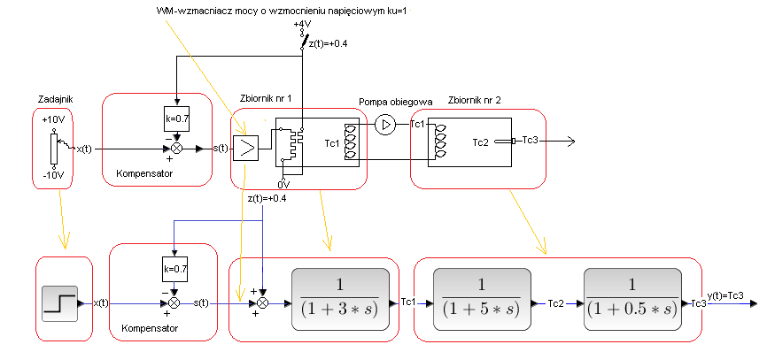
Fig. 30-3
The diagram above is Fig. 30-1 + additional compensator block. It measures the voltage (i.e. disturbance z(t)=+0.4) and then calculates the control signal s(t)=x(t)-k*z(t) which is fed to the input of the object. The control signal s(t) due to the subtraction operation has the opposite direction to the disturbance z(t). If the disturbance heats (as in the diagram), then s(t) reduces the power supply to the heater, i.e. it cools it down. If the disturbance cools, then s(t) additionally heats. The compensator therefore functions as a controller.
Some people call it a feedforward controller. It’s a strange controller. It does not use the output signal y(t), only the input signals, i.e.:
– x(t) (which is normal for any controller)
– disturbance z(t) (this is the wonder!).

Fig. 30-4
The response to x(t), i.e. the time chart of y(t) in 3…40 seconds, is obvious. In 40 sec there was a disturbance z(t)=+0.4 – additional heating. The control signal s(t) reacted correctly, it decreased the heating by 0.7*0.4=0.28 to the value of 0.72. In total, a power of 0.72+0.28=1.12 is delivered, which corresponds to a steady state temperature of y(t)=+112ºC. Compared to Fig. 30-2, where there was no compensation, the disturbance z(t) was partially suppressed. You don’t need to be a genius to predict the effect of full compensation. Full disturbance suppression z(t) will be ensured only by full compensation k=1.
Chapter 30.3.3 Opened loop with the complete noise compensation k=1

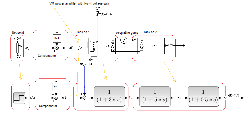
Fig. 30-5
Compensation factor k=1. Can you guess the effect of full compensation?

Fig. 30-6
The control signal s(t) is now in anti-phase to z(t) and the disturbance has been fully compensated. The output signal y(t) despite the disturbance z(t)=+0.4 (additional heating) will not budge. It stands like a Uhlan lance. There are 2 questions here?
1- Why didn’t we give the compensation factor k=1 right away?
2- Since there is 100% disturbance suppression, why is it not a universal method.
Answer no 1
It was easy for us because we know the object’s transmittance Go(s) and k=1 was obvious. But on a real object, e.g. in the Refinery, you don’t see the transmittance, only some column, heating pipelines and those not fully worked out “disturbance” signals. Even if you have a compensation potentiometer on the controller, e.g. k = 0 … 1.5, you will select the ideal value either experimentally by turning the potentiometer, or theoretically, when you have a thoroughly mathematically worked out object. Returning to the “k potentiometer“, in serious systems it appears only as software. The operator “turns” it through the keyboard, entering the appropriate numbers into the system.
Note*
Earlier, there were systems where, despite z(t) disturbance, the PID controller worked so that the red y(t) “stood” in place. However, this was only due to the small gain of the oscilloscope. If it was larger, the red y(t) would “move”.
Answer to 2
Actually. So far, we have not encountered such a perfect suppression of disturbance. But the compensation is successful only when we know the object well, the disturbance z(t) can be measured and the parameters of the object are constant in time. And that’s not always the case. In addition, the system is not immune to other disturbances! Therefore, in chapter. 30.5 you will learn about the Closed-Open Systems, in which there is a compensator that suppresses the measured disturbance and a simple feedback that suppresses the remaining disturbances.
Chapter 30.3.4 Opened System with “normal” Compensation for disturbances “in the middle” of Go(s)
Disturbance in the “center of the object”, but compensator k=1. As in the diagram below.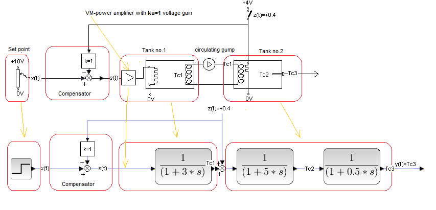

Fig. 30-7
The “disturbance” heater is right next to the tank 2 coil. We expect the disturbance z(t) to be compensated to some extent. The response should be better than the uncompensated system in Fig. 30-2. But is it as good as in Fig. 30-6 with disturbance at the beginning of the object?

Fig. 30-8
During 3…40 seconds, the output signal y(t)=Tc3 is the same as in Fig. 30-3, 6 and 9 because there was no disturbance yet. In 40 sec z(t)=+0.4 occurred from the “disturbance” heater. The compensator reacted correctly by lowering the control signal s(t) also to 0.4 – in antiphase. But this time you can see the impact of the disturbance z(t). Transitional indeed. Why?
Because the decrease in the inflow of heating power to tank 2 did not occur abruptly, but with an inertia of 3 seconds, as the temperature Tc1 in tank 1 equals the temperature of the liquid in the coil of tank 2. After 65 sec. the output signal returned to its initial state y(t)=+100ºC. The compensator finally did its job, though not as gloriously as in Fig. 30-5, where z(t) acted directly on the input. Then the disturbance was attenuated perfectly immediately by a decrease in the heating power of the heater in tank 1.
It’s good, but we want it to be even better. How? For example, you can put an additional electric heater with a Peltier element right next to the disturbance heater. Then the negative Peltier voltage will cause cooling, i.e. it will cause an immediate drop in the thermal power delivered to tank 2. This is a solution, but it comes with additional structure and cost, compromising energy efficiency.
The existing heater in tank 1 can also be used. Note that the imperfection of disturbance suppression z(t)=+0.4 is due to the fact that the disturbance transmittance between z(t) and sk(t) is
Gzk(s)=1/(1 +sT) where T=3 sec. So it is an inertial unit with constants k=-1 and T=3 sec. What about making it a proportional unit Gzk(s)=1? Then it would be possible to completely suppress the disturbance, as in Fig. 30-5. Just how to do it?
Chapter 30.3.5 “Reverse” transmittance

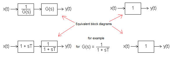
Fig. 30-9
How to make any G(s) term proportional G(s)=1?
Theoretically, it is very simple. G(s) should be preceded by its inverse. Just like 2 amplifiers connected in series with gains k1=0.1 and k2=10 give a gain k=k1*k2=1.
And what does it look like when G(s) is e.g. an inertial unit?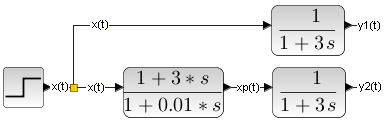

Fig. 30-10
From the inertial unit G(s)=1/(1+3*s) we want to make a proportional unit G(s)=1. As we have shown in Fig. 30-9, it should be connected in series with the inverse G(s), i.e. with the unit (1 + 3s). Right away. and what is it doing here in the denominator (1 + 0.01s)? Oh yeah. It is difficult to realize the perfect (1 + 3s). It gives infinity as a response to the step x(t), because the speed of the jump increase is also infinite.
Therefore, we will put 1 + 0.01s in the denominator. This corresponds to a series connection (1 + 3s) with an inertial unit with a very small time constant T=0.01 sec, i.e. 1/(1 + 0.01*s). The response y2(t) to step x(t) should be “almost a step”, not a perfect jump. Let’s check.

Fig. 30-11
– y1(t) response of the inertial unit
– y2(t) response of the “almost” proportional term G(s)=1 as the product of the inertial unit and its reciprocal.
Note
In a moment it will turn out to be the “almost proportional” unit.
At the first moment, y2(t) perfectly coincides with the step x(t). But if you look closely, the red y2(t) in 1 second does not coincide with the x(t) step. Rather, there is a very rapid increase to y2(t) as in the inertial unit with a very small time constant. This is where the impact (1+0.01*s) in the denominator is! Therefore, y2(t) is the answer of the “nearly proportional” unit.
And why does y2(t) increase very quickly during the step compared to the response of y1(t) of the inertial unit alone? Then look at how powerful the xp(t) signal is at the input of the inertial unit. The xp(t) signal is cut off by the oscilloscope, but it reaches the value xp(t)=301! Then it drops very quickly to 1. Such a time chart xp(t) causes a very rapid increase in the signal y2(t) to the value y2(t)=1.
Conclusion
A differentiating unit appeared in the nominator of the compensating element, which causes large instantaneous value–> xp(t)=301! This requires the provision of large temporary power, which can be quite troublesome. Even stronger differentiations – read second and higher derivatives – occur with more complex objects than inertial ones. Despite this, compensation often improves disturbances suppression, even when supply voltages are limited. Especially with simple dynamic objects.
Chapter 30.3.6 System with “inverse” compensation of disturbances “in the middle” of Go(s)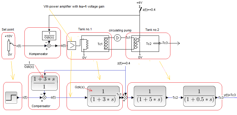

Fig. 30-12
Below is the system model. The only difference is the denominator of the compensator (1 + 0.01*s) introducing a small inertia. It prevents diracs – infinitely large pins when jumping. The pin will remain, but of finite value! It does not significantly negatively affect the attenuation of disturbance z(t). Let’s agree that this is reverse compensation, although formally it is not.

Fig. 30-13
Until the disturbance z(t)=+0.4, in 40 seconds, the compensating element has not yet joined the action, i.e. the time charts are the same as in Fig. 30-11. It is clearly visible how the x(t) step is ahead of Tc1 and Tc1 is ahead of y(t)=Tc3. Let me remind you that Tc1 as the temperature in the coil of tank 2 is the input signal to this object, and y(t)=Tc3 (temperature measured with a thermometer) is the output signal.
In 40 seconds, a disturbance z(t)=+0.4 (additional heating) appeared, but y(t) did not even move! Great, compare it with Fig. 30-8 where there was “normal” compensation, otherwise “without reverse transmittance”. A little comment here. However, it “twitched” a bit, because this is not a perfect reverse compensation. But an insensitive oscilloscope doesn’t show it.
Further analysis is difficult:
Firstly
The oscilloscope “cuts”. The control signal s(t) got a negative kick in 40 seconds -> negative pin about -120! This is the differentiation effect of the compensating unit. And only thanks to a small inertia (the denominator of the compensator) the pin is not a dirac with a minus infinity signal. In fact, the pin is slightly stretched in time as in Fig. 30-11.
Secondly
the time charts partially overlap, therefore in Fig. 30-14 the following are shown separately:
– Temperaturein the coil Tc1  the input signal to the tank 2
– disturbance z(t)=+0.4
The control signal s(t)=-120 in 40 sec is a temporary powerful cooling of the Peltier heater-cooler. Now the temperature Tc1 in the tank 2 coil  will drop almost immediately, thus compensating for the disturbance heater z(t)=+0.4.

Fig. 30-14
Thanks to the compensator, the input signal s(t), (actually its negative “cooling” pin Fig. 30-13), the temperature Tc1 of the tank 2 coil will be almost “negative rectangular”. And this will almost perfectly compensate for the disturbance z(t)=+0.4. Recall that Tc1 is the input for tank 2. This is all clear from animation Fig. 30-13. And even more in Fig. 30-14 where there are only Tc1 and z(t)=+0.4 time charts.

Chapter 30.4 Closed System
This is the most commonly used control scheme. You can say that everyone else is just a modification of it.
For example:
– Open System is a Closed System with a broken loop
– Open System with Compensation is Closed System + Compensation with a broken loop
–Cascade Control is a combination of two Closed Controls.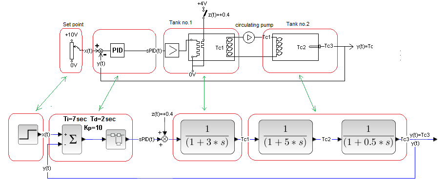

Fig.30-15
Closed System.
This is a copy of the Fig. 29-10 from Chapter 29. The open object – Heat Exchanger controlled from the 0…+10V potentiometer, was closed with a negative feedback loop with the PID controller. This is the end of the topic, because the entire course is about Closed Systems.

Chapter 30.5 Closed System with Compensation – another name Closed-Open System
Chapter 30.5.1 Introduction
An Open System with Compensation can completely suppress the disturbance z(t), which can be measured as in Fig. 30-5. It is, of course, vulnerable to other uncompensated disturbances, such as the “disturbance” heater at the coil in tank 2. The solution suggests itself. Close the system with a feedback loop with a PID controller. We expect this to result in perfect disturbance suppression with full compensation and normal disturbance suppression.
We will explore different combinations:
– Full compensation k=1 with disturbance on the object input –>chapter 30.5.2
– Incomplete compensation k=0.7 with disturbance at the object input–>chapter 30.5.3
– Full compensation k=1 with disturbance in the “center” of the object–>chapter 30.5.4
– Full compensation k=1 with disturbance at the input of the object and with additional disturbance in the “center” of the object–>chapter 30.5.5
Chap. 30.5.2 Full Compensation k=1 with disturbance at the object input

Fig. 30-16
The Full Compensated System from Fig. 30-7 after closing the loop with the PID controller.
Kp, Ti, Td settings provide optimal response to x(t) step.

Fig. 30-17
Up to the disturbance z(t)=+0.4 in 40 second, the response to the step x(t) is identical to that of the Closed System–>Fig. 29-11 from chapter 29.
In 40 seconds, the disturbance z(t)=+0.4 caused an immediate reaction of the compensator in the opposite phase in the form of a decrease in the signal s(t) also by 0.4. The disturbance z(t) was thus fully compensated. The output signal y(t) didn’t even budge (because the PID “thinks” there was no disturbance!) and the error e(t) still remained zero.
The control signal s(t) is the sum of the PID->sPID(t) controller and the compensator signal. Only the compensator signal reacted to z(t)=+0.4.
Chap. 30.5.3 Incomplete Compensation k=0.7 with disturbance at the object input
We try to make everything perfect, including compensation. But it doesn’t always work, for various reasons. The disturbance z(t) may be difficult to measure, for example… This corresponds to the case where, for example, k=0.7 and not k=1.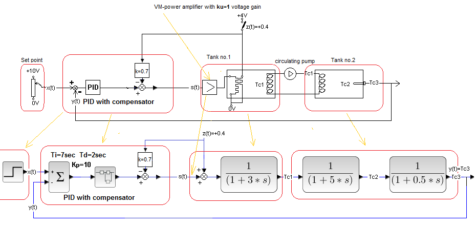

Fig. 30-18
Almost a copy of Fig. 30-16. The only difference is k=0.7 and not k=1. So we expect that there will be some disturbance effect on the output y(t).

Fig. 30-19
Up to 40 second the response to the x(t) step is of course the same as before. However, from 40 second only part of the disturbance z(t)=+0.4 ie 0.7*0.4=0.28 is immediately compensated by the compensator. The rest, i.e. 0.4-0.28=0.12, is suppressed by PID and therefore not immediately! It lasts over 10 seconds, which can be seen in the time chart s(t). All in all, y(t) is not perfectly damped as with full compensation, but it is clearly better than the system with feedback without compensation –>Fig. 29-11 from chapter 29. The response is as if it were a feedback system with no compensation, but with less disturbance. z(t)=+0.12 ( and not z(t)=+0.4)
Chapter 30.5.4 Full compensation k=1 with disturbance in the “center” of the object
It will arise when the open System with “Inverse” Compensation from Fig. 30-12 is closed with a feedback loop with the PID controller.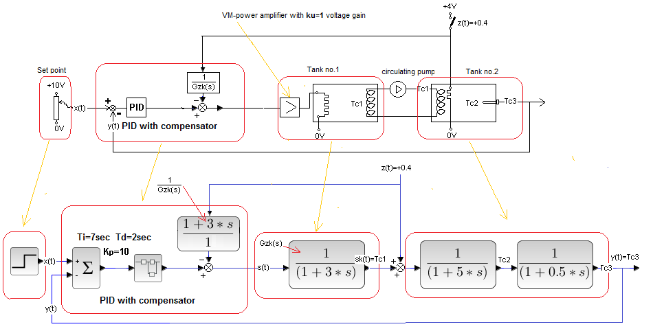

Fig. 30-20
Closed system with full compensation and with a disturbance in the middle of the object.

Fig. 30-21
Until the disturbance z(t)=+0.4 in 40 seconds, the response to the x(t) step is the same as for the Closed System->Fig. 29-11 from chapter 29. Just at this time z(t)=0, i.e. the “compensating part”, does nothing. In 40 seconds, z(t) appeared at the coil of tank 2, which was immediately* compensated by the signal Tc1. Therefore, z(t)=+0.4 was not “noticed” by the PID and the response y(t) is the same as for a closed system without disturbance!
Note
In 40 seconds, a negative pin s(t) appears, exactly as in Fig. 30-13. This makes the temperature signal almost perfectly rectangular. The oscilloscope didn’t show it.
Chapter 30.5.5 Full Compensation  k=1 with disturbance at the input of the object and with additional disturbance in the “center” of the object
It will be a Closed System with Full Compensation from chapter 30.5.2 with an additional uncompensated disturbance. A compensated heating disturbance z1(t)=+0.4 will occur as usual in 40 sec. and uncompensated cooling disturbance z2(t)=-0.6 in 55 sec.

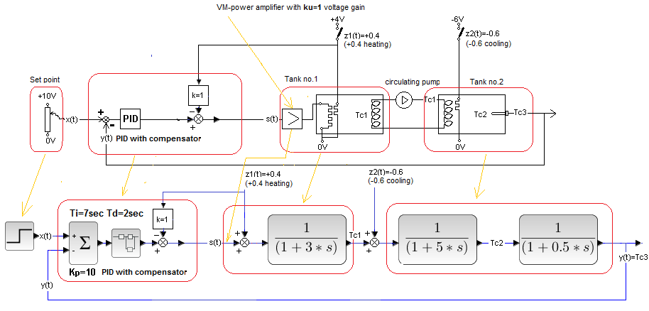
Fig. 30-22
The cooling disturbance z2(t)=-0.6 right next to the tank coil 2 is caused by a negative voltage spike of -6V in 55 seconds. I remind you that the heater is the so-called Peltier element, where positive voltage heats and negative voltage cools.

Fig. 30-23
Until the disturbance z1(t)=+0.4 in 40 sec, the response to the x(t) step is identical to that for the Closed System without compensation. It’s just that during this time z1(t)=0, i.e. the “compensating part”, it does nothing, as if it were not there. In 40 sec additional heating appeared z1(t)=+0.4, which was immediately compensated by the signal s(t). Therefore, y(t) itself did not change and the PID controller did not even react. So until then the system behaves as in Chap. 30.5.2.
As for the “cooling” disturbance z2(t)=-0.6, as it was uncompensated, it was suppressed with the usual PID feedback. Except that for the PID itself it was only a disturbance z2′(t)=-0.6+0.4=-0.2! Because the disturbance z1(t)=+0.4 was already taken care of by the compensation part of the controller k=1.
Chapter 30.5.6 Conclusions
1. A Closed System with Compensation can theoretically (!) perfectly suppress a disturbance, provided that:
– accurate disturbances measurement
– selection of the appropriate transmittance of the compensator. This involves a thorough knowledge of the Go(s) object.
When the disturbance is at the input of the object, the transmittance of the compensator is
k=1–>chapter 30.5.2
When the disturbance is in the “center” of the object, it is the inverse transmittance
1/Gzk(s)–>chapter 30.5.4
2. Even when it is not possible to accurately measure or select the ideal compensator, the quality of control is significantly improved.–>chapter 30.5.3. This also applies to the inverse transmittance when the disturbance is in the “center” of the object.
3. In the inverse transmittance there is an s in the numerator (causing a strong differentiation of the signal. It is difficult to realize (infinite instantaneous power) and therefore the practical results are not as beautiful as in our experiments. But even then there is a clear improvement in control quality.
4. Other uncompensated disturbances are suppressed by PID by ordinary feedback–>chapter 30.5.5

Chap. 30.6 Cascade System
Chap. 30.6.1 Introduction
The system allows better suppression of a specific disturbance than the classic Closed System and a little worse than the Closed System with Compensation. Contrary to the latter, it does not require measurement of the disturbance, nor such precise knowledge of the Go(s) object.
The principle is similar to the organization of an enterprise. The director assigns a task to be performed by the menager of the subordinate department and ceases to be interested in it. He does not investigate the disturbances affecting the ward, whether mr, Smith came drunk or the Client did not pay the invoice. For the director, the monthly plan is to be completed. Information about a disturbance reaches the manager faster than the director, and therefore he has greater possibilities to suppress it. He will use the method of the stick (threat of dismissal) and the carrot (bonus). The manager will eliminate the disturbance faster than the director. In the Cascade System, the role of the director is performed by the master controller – most often PID, and the manager is the slave controller – usually P type.
Chap. 30.6.2 Cascade System with one disturbance
More precisely, with a disturbance or even several affecting a certain part of the object.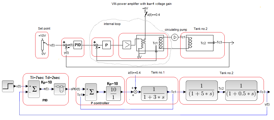

Fig. 30-24
Cascade system with disturbance
The P controller compares the temperature Tc1 of the tank 1 liquid with the PID output signal. So an inner loop was created – an ordinary closed system, in which the Tc1 output signal “tries” to imitate the signal from the PID. It is clearly visible which regulator is the director of the entire company – 2 tanks, and which is only the manager of tank 1.
So PID is the master controller and P is the slave controller. Sometimes the subordinate is PI or even PID.
The disturbance z(t)=+0.4 is the activation of the auxiliary heater located at the control heater of tank 1. Compare this diagram with the usual Closed System in Fig. 29-10 chapter 29 . When we break the internal feedback loop from Tc1 and replace the P regulator with a bare wire, we get an ordinary Closed System. From Fig. 29-11 chapter 29 it can be seen that the disturbance of a normal closed system has been completely suppressed.
And what to expect from the Cascade System?
Firstly
– The inertia of tank 1, which has been covered by a strong feedback, will decrease –>Kp=10. Therefore, the inertia of the entire object will also decrease and it will become easier to control. So it should give a shorter response time to x(t) step than classical feedback.
Secondly
– The disturbance attenuation z(t) will improve dramatically. Before the PID reacts, the P controller will do it much faster! After all, it only has to do with one inertia of tank 1.
I will say more. The P controller will suppress z(t) so quickly that the PID will barely notice the change in y(t). The main work of suppressing disturbance z(t) will be done by the slave controller P and the master PID will only finish it.
Let’s check it.

Fig. 30-25
The output is red y(t). Compare with the response of a classic closed system–>Fig. 29-11 from chapter 29. Suppression of z(t) super as if it wasn’t there, but the response to the x(t) step is a shame to talk about. It’s easy to explain. Simply, the controller settings Kp=10 Ti=7 sec. Td=2 sec. have been selected for the system shown in Fig. 32-11 from chapter 32. And as I wrote in the introduction, the inertia of the object in Fig. 30-24 is smaller, because the inertia of tank 1 covered by the inner loop has almost disappeared. Conclusion -> there will be other optimal settings. Let’s check.
Chapter 30.6.3 Cascade with one disturbace and with more optimal settings
The settings of the PID controller, i.e. Kp=10 Ti=5 sec and Td=0.55 sec, were selected by trial and error. Although they may not be fully optimal, there should be a clear improvement in time charts.

Fig. 30-26
Recall that the output is y(t)! Shocking. And if you compare it with the response of a classical closed system Fig. 29-11 from chapter 29, it’s a megashock! One more thing. For example, see Fig. 30-25, where the steady state was s(t)=y(t)–> the control signal at the input of the object s(t) equaled the output signal y(t). We got used to “it’s always like this”. And in Fig. 30-26 it is not (here instead of s(t) there is sPID(t)). How to explain it? The matter is simple. In general, it is always the case that in the steady state there is s(t)=k*y(t), where k is the static gain of the object with the controller. Let me remind you that the steady state is the state of equilibrium found by the controller. When s(t) is too large, the controller will reduce y(t) and vice versa. So far with normal feedback, it’s mostly k=1, and then it’s always s(t)=y(t)?
And what about cascade control in Fig. 30-24? Is the gain of the object between the signals sPID(t) and y(t)=TC3 equal to k=1?
NO! because the inner loop around the tank 1, closing by the P controller, caused Kz=0.909. Such amplification “sees” the master PID controller.
And this means that in steady state y(t)=0.909*sPID(t) or sPID(t)=1.1y(t). This is confirmed in Fig. 30-26.
Chapter 30.6.4 Cascade with two disturbances

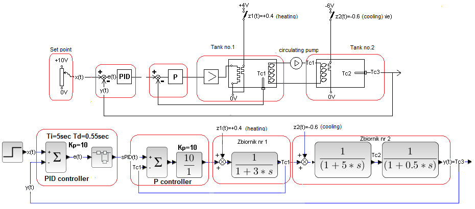
Fig. 30-27
The disturbance z1(t)=+0.4 is additional heating entering the inner loop. Which is exactly the same as z(t)=+0.4 in previous experiments. Therefore, we expect it to be very strongly damped as well.
The disturbance z2(t)=-0.6 is cooling (minus the Peltier!) of the input coil to tank 2. It is subject to ordinary feedback. The disturbance should also be completely suppressed, although not as fast as z1(t).

Fig. 30-28
Up to 55 sec, i.e. until z2(t) appears, the response is for obvious reasons identical to Fig. 30-26. The disturbance suppression z1(t) is so strong (so good!) that there is no visible effect on the output signal y(t). Although there is, but the oscilloscope does not show it.
In 55 seconds, a disturbance z2(t)=-0.6 occurred – cooling at the tank 2 coil. The PID controller reacted correctly by increasing the power of the tank 1 heater. The influence of the disturbance z2(t) is already visible here, although it was also completely suppressed. Did the P slave controller have any (positive!) effect on the disturbance suppression z2(t). I think so. After all, the internal feedback involving tank 1 seems to have reduced its inertia. Now almost all the inertia of the two tanks is only in tank 2. And objects with smaller inertias are easier to control.

Chap. 30.7 Ratio Control System
Chap. 30.7.1 Introduction
The output signal y(t) of the ordinary Control System tries to follow the input signal so that in steady state y(t)=x(t). The Ratio Control System does a similar job, just according to the formula y(t)=k*x(t).
It can be used, for example, in the Paint Mixing Plant–>Chapter 30.7.2, where a new paint will be created by mixing two different ones. It is known that the color depends on the ratio of their mixing. So it is enough to fill the mixing tank with 2 flows of two paints, e.g. red and green, whose flows are related by the relationship red=k*green.
Another application is the Steam Boiler–>Chapter 30.7.3. It is known that optimal combustion depends on the right ratio of gas and air. It’s bad when there’s too much gas. Then not only will not everything burn up -> low efficiency, but the environment will be polluted. And when there is not enough gas? It is true that everything will burn, but the excess air unnecessarily cools the boiler and heats the atmosphere, reducing the energy efficiency of the boiler. It is therefore necessary to ensure an optimal ratio of gas and air flows.
Chapter 30.7.2 Paint Mixing Plant
It is a good example of the application of the Ratio Control System. The right color is the right mix of three colors, here for simplicity only two red and green. We want a color where green/red=1/3. So it is enough to fill the tank with 2 flows from the pipelines – green and red, for which the ratio of flows.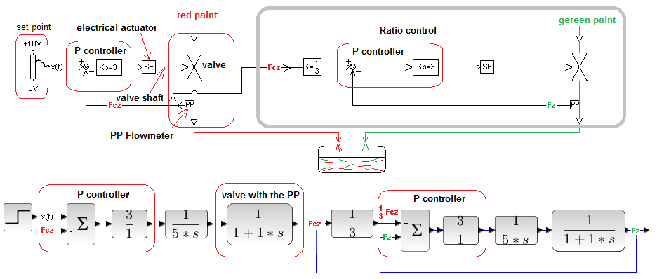

Fig. 30-29
Technological and control diagram of the mixing plant

But first let’s talk about valves. You can leave if you know the topic.
The Ratio Control System is most often associated with flows. The flows in the pipelines are controlled by valves. Therefore, to begin with, the absolute minimum of knowledge. Everyone has it at home. A closed valve means no flow, an open valve means maximum flow limited only by the pressure in the network, the hydraulic resistance of the piping and the resistance of the fully open valve itself. By turning the tap, I set the indirect flow, i.e. I have the ability to control it.
The most important feature of each valve is the so-called Kv factor. I will not go into details further. I will just say that a small tap in the house is small Kv, and a large valve on the industrial pipeline is large Kv.
The second feature is its characteristics, i.e. the function between the shift of the valve stem (at home it is the angle of rotation of the tap) and the flow F. It would seem that with unscrewing the valve, the “hole”, i.e. the surface through which the liquid flows, should increase proportionally from 0 (closed) to MAX (open). So that the flow also increases in a linear way, which is the most desirable in control. But it’s not like that! At first, the area increases slowly and then faster and faster. Something like an exponential function. This is the so-called equal percentage characteristics. It turns out that just such non-linearity will provide (approximately) a linear characteristic of the valve, when the input is the movement of the valve stem (and plug) and the output is flow. How to explain it?
At the beginning there is a small “hole”, but the liquid has a terrible desire to flow through it, because there is a large pressure drop between the two sides of the “hole”. Then the surface area increases, but the desire to flow decreases because the pressure drop decreases. Overall, the increase in surface area and the decrease in pressure work against each other and the characteristic becomes more linear.
From the above, it follows that when selecting a valve, you must select:
a-Kv such that for x(t)=1 (+10V on the potentiometer) the valve is fully open -> maximum flow
b-valve with equal percentage characteristics
ad.a
-When Kv too large, it will open only, for example, up to 10%, giving the maximum flow limited by the resistance of the external piping – it’s a pity for a large valve when you can give a smaller one, i.e. cheaper.
-When Kv too small, it will open almost immediately to 100%, then it works as a permanent choke, although the pressure of the network and piping could give a greater flow.
ad.b
-Provides the desired linearity in automatics

How does the mixer work?
With the adjuster – potentiometer 0…+10V, we set the maximum flow Fcz of the red paint, which is measured with the flow converter PP. The maximum flow also corresponds to +10V at the output of the PP converter. The P controller compares the setpoint value x(t) with the current flow and generates an appropriate control signal for the SE electric actuator. This signal moves the valve stem at a rate proportional to the voltage from the controller. Positive voltage opens the valve, negative voltage closes it, and zero voltage disables it. So valve+actuator is a typical integrating unit with a transmittance of 1/5s. The number 5 in the denominator means that at +10V, but without feedback, the valve will open to the max within 5 sec*. The valve with the PP converter is an inertial element with a time constant T=1 sec. The pipeline with red paint + automatics form the I – i.e. integrating control system. Control I was discussed in detail in Chapter 28. The green part works in a similar way. Here, in turn, the set value is the flow 1/3*Fcz. We expect that in the steady state the flow Fz will be 3 times smaller than z Fcz. Let’s check.
* the s symbol in the 1/5s transmittance is not a second, but a complex number s, as it happens in transmittances.

Fig. 30-30
The goal of the Ratio Control has been achieved. The green Fz flow in steady state is one third of the red Fz.
Chapter. 30.7.3 Steam Boiler
It is a less trivial example of a Ratio Control than a Paint Mixing Plant.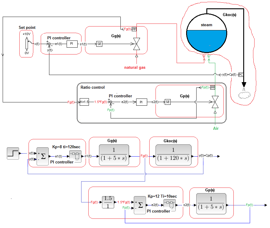

Fig. 30-31
Technological and block diagram of a typical Steam Boiler.
It is a drum filled with water and heated with natural gas. Supplies various devices not shown in the diagram with steam. The automatics tries to maintain a constant steam pressure at the boiler outlet cp(t) regardless of disturbances, which may be, for example, switching on an additional steam receiver. 
Gas needs air, more precisely oxygen. Optimum combustion ensured at a certain ratio of air flow to gas flow.
If it is too small, not all the gas will be burned –> lower efficiency and environmental pollution.
If it is too large, the unburnt air cools the exhaust gases unnecessarily –> lower efficiency.
Boilers are not my field, but k=10 is supposedly optimal. To make the graphs of gas and air less different from each other, for didactic reasons we will assume that k=1.5.
Now let’s look at the schematic from the automatics point of view. We distinguish the following dynamic blocks in it.
Gkoc(s)-Steam Boiler 
Input – gas flow Fg(t) and k=1.5 times the air flow Fp(t)*
Output – pressure Cp(t) on the pipeline. More precisely, it will be the voltage, where 0…10V is 0…10 MPa.
The physics here is very simple. We assume that by some miracle the water level is kept constant regardless of the steam discharge. This is usually done by a very precise and fast level control system. It provides fluctuations of less than 1 cm! And the steam keeps going!
This is where Cascade Control comes into play. It is also possible, by additionally measuring the water inflow to the drum and the steam outflow, to accurately calculate the disturbance affecting the level. That is Closed System with Compensation.
These were just side notes. So we’re still stuck with the constant-level miracle. An increase in the gas supply Fg(t) and Fp(t) increases the temperature and thus the pressure Cp(t) of the steam. Of course, not immediately, but just like the inertial unit with a time constant T=120 sec, subject to negative feedback.
*Fp(t) flow is only shown in the top drawing at the drum. However, it is not shown in the lower figure as an input to Gkoc(s). And rightly so, because the vapor pressure Cp(t) depends only on the flow Fp(t), assuming that Fp(t)=k*Fg(t).
Gg(s)-Gas Control Block 
Input – control signal s1(t) from the PI controller
Output – gas flow Fg(t)
SE-Electric Actuator – Unlike the SE actuator in the Mixing Plant, it is a proportional and not an integrating unit. So it has (not shown in the diagram) internal feedback from the position of the stem. Cascade Control is bowing again -> there will be better time charts.
PP–flow transducer converts the flow signal Fg(t) to 0…10V.
Valve–Stem displacement changes into an increase in the flow surface, i.e. a change in flow. The designer selected the appropriate valve size->Kv and equal percentage characteristics to achieve linearity. We assume that Gg(s) is an inertialunit with a time constant T=5 sec.
Type PI Pressure Controller
It constantly compares the pressure Cp(t) with the setpoint value x(t).
When Cp(t) increases, the error e1(t) decreases–>Fg(t) decreases, the water temperature  and steam pressure Cp(t) decreases.
When Cp(t) decreases, the error e1(t) increases–>Fg(t) increases, water temperature and steam pressure Cp(t) increases.
In this way, the controller tries to keep the pressure Cp(t) constant equal to the setpoint value x(t). The PI control will ensure zero error and good time charts.
Gp(s)-Air Control Block
Input – control signal s2(t) from the PI controller
Output – airflow Fp(t)
Operation and dynamics the same as Gg(s) – Gas Control Block
PI Flow Controller
The setpoint is k*Fg(t). Therefore, the controller tracks the airflow ensuring Fp(t)=k*Fg(t).
Let’s see how the whole system works.

Fig. 30-32
The goal of control the has been achieved. In steady state, the air flow is 1.5 times greater than the gas flow. I emphasize that the flows of gas Fg(t) and air Fg(t) are only auxiliary signals here. The most important is the steam pressure Cp(t).