Automatics

Chapter 3 Inertial Unit
Chapter 3.1 Introduction
This is the simplest dynamic unit except Proportional. Unit step response is no longer instantaneous. You may not know the concept of transfer function-transmittance G(s) yet, but after completing this chapter you will associate its parameters with time courses. To treat the transfer function G(s) as a kind of amplification, no differential or operator calculus is needed. Maybe that was too strong a word. It would be better that way. Knowledge of higher mathematics is not absolutely necessary to understand automatics, but it is very helpful.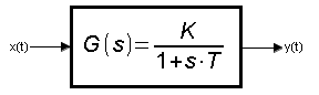

Fig. 3-1
Inertial unit parameters:
–K -steady state gain
–T – time constant
We will do some experiments with different T  time constants.
We will do some experiments with different input signals x(t). The output signals y(t) will be observed on the bargraf or on the oscilloscope.

Chapter 3.2 K=1 T=5 sek, step x(t) from slider, y(t)  bargraf

Fig. 3-2
Response to a unit step of the inertial unit K=1 and T=5sec
The x(t) input signal was set with a 0-1 step on the slider.
You can follow the waveforms:
analog -x(t) on the slider and bargraph
digitally -y(t) on gauges
Digital meters are especially useful for slow changes at the end of the waveform.
Note
The second is only accidentally associated with the complex number s at the time constant T.
What if we increase the time constant to T=10 sec?

Chapter 3.3 K=1 T=10 sek, step x(t) from slider, y(t)  bargraf

Fig. 3-3
Response to a unit step of the inertial unit K=1 and T=10sec
Compare with waveform Fig. 3-2. The “heaviness” of the transmittance is clearly 2 times greater.

Chapter 3.4 K=1 T=5 sek, step x(t) from slider, y(t)  oscilloscope

Fig. 3-4
Response to a unit step of the inertial element K=1 and T=5sec
The input signal x(t) is a step unit that occurred in 12 seconds.
The output signal y(t) has the highest rate of increase at the beginning.  Then it increases, but at a decreasing speed. In a steady state, it reaches the value y=1.
The waveform clearly shows what is what in the transmittance G(s) in Fig. 3-4.
1 in the transmittance numerator G(s) is the steady-state gain K=y/x=1.
5 in the transfer function denominator is the time constant T=5 seconds.
This is the time after which the steady state y(t)=1 would occur if the growth rate was still the same as at the beginning. The signal would then grow like a tangent – a dotted line. The state y(t)=x(t)=1 would be reached after T=5sec=17sec-12sec.
You can read the times 17sec and 12sec from the time axis t.

Chapter 3.5 “Smoothing” action of the inertial unit K=1, T=5sec
We “swing” the slider. So we will check how the inertial term behaves to fast changes of the input signal x(t).

Fig. 3-5
“Smoothing” action of the inertial unit
Note:
There is a relatively large inertia T=5sec. Therefore, the output signal y(t) is hardly similar to the input one.
It will become more like when:
– the x(t) signal is slowly changing
– the time constant T will be smaller, e.g. T=0.2sec

Chap. 3.6 Comparison of two different inertial units
The same unit step x(t) will be given to 2 different inertial units.
This time x(t) comes from a signal generator that is more precise than the previous slider.

Fig. 3-6
The inputs of two inertial units, in which parameters 3 and 7 are “replaced”, are supplied with a unit step x(t).
In Fig. 3-4 we had an inertial unit in which K=1 and T=5sec. When K=1 then y(t)=1. We also showed how to calculate T=5sec from the graph.
Now we calculated K1=7 and T1=3 sec for the upper inertial term and K2=3 and T2=7 sec for the lower one in the same way.

Chapter 3.7 Dirac pulse
Chapter. 3.7.1 Introduction
Another signal used in the control theory is the so-called Dirac pulse–> x(t) = δ(t). Its characteristic feature is that it lasts infinitely short but has an infinitely high value. However, the energy of this impulse, i.e. the impulse field, is equal to unity, i.e. it is finite.
An approximation can be, for example, a power plant that supplies an electric kettle with all its power (e.g. 3600 MW), but for a very short time. The water in the kettle will heat up to +100°C because in a few nanoseconds, finite energy will be delivered (and not a lot at all!), and the kettle will not be destroyed!
For us, the kettle got hot immediately! We think we are dealing with Dirac’s Ideal pulse.
A mechanical example of a Dirac pulse is a hammer blow. It also takes a very short time and during this time the finished work of driving the nail will be done.
Conclusion There are no ideal Dirac Pulses in nature. There are only real approximations of it.

Chapter 3.7.2 Inertial unit K=1 T=1sek with the real Dirac pulse

Fig. 3-7
Inertial unit response to (almost) Dirac pulse δ(t)
A pulse with an amplitude of A=10 and a duration of tp=0.1sec is only an approximation of the ideal Dirac pulse δ(t). You can see how the signal grows rapidly over time tp. Then it drops because there is zero in the input. This is how fast charging through the resistor R of the capacitor C and its discharge looks like.

Chapter 3.7.3 Inertial unit K=1 T=1 sec with “more ideal” Dirac pulse
The previous Dirac with an amplitude of 10 lasted 0.1 seconds. Since we are unable to give a perfect Dirac, let’s at least give something closer to the ideal. i.e. pulse with an amplitude of 100 that will last 0.01 sec. Notice that its energy, or pulse area, is also 1.

Fig. 3-8
Inertial unit response to a (more ideal) Dirac pulse δ(t)
The pulse is 10 times higher (i.e. 100 and exceeds the scope of the oscilloscope) and 10 times narrower. Its field=1, or energy, is the same as before. It’s still not perfect, although Dirac’s appearance is textbook.

Chapter 3.8 Why do we need these Diracs?
Especially since a unit step  is technically easier to implement than a Dirac pin. In the unit step, it is enough to enter the maximum power per input, e.g. 100 kW. In an almost perfect Dirac, this is Power Station 4,000 MW for a few nanoseconds. There are technical ways to deliver a short pulse of high power without the use of a power plant, e.g. laser power supplies, radar stations … But this is no longer simple.
Exactly. Why this Dirac? I’ll run a little ahead. It turns out that the transfer function G(s) is simply the Laplace transformation of the response y(t) to the Dirac pulse. That’s all for now. A special chapter will be devoted to G(s) and Laplace transforms.

Chap. 3-9 Two seemingly different inertial units

Fig. 3-9
The same unit step x(t) acts simultaneously on the lower and upper inertial units. The reactions, i.e. y1(t) and y2(t) are identical. So both inertial units are also identical. But in the upper member you can’t see the parameters K=2 and T=3sec. To see them, make the upper denominator 1+… So divide the upper numerator and denominator by 7. It turns out that both fractions G1(s) and G2(s) are the same 1/(1+3*s)!
This lower transmittance is in the normalized version. It is easy to read the parameters K=2 and T=3sec. All basic dynamic units from chapters. 2…9 are presented in a normalized version. Especially in chapter 7 Oscillatory Unit.

Chapter 3.10 Typical inertial units
RC Circuit
We’ll start with an example of an electric-RC circuit. When I apply a voltage unit step x(t) to the input, the voltage y(t) with such a waveform will appear at the output.

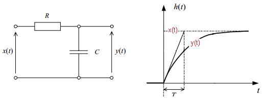
Fig. 3-10
It is an Inertial unit with parameters k and T, k=1 because in steady state y(t) = x(t) When, for example, R = 100 kΩ and C = 10 µF, then T = R*C = 100,000 Ω * 10* 0.000001F = 1 second
DC motor
If  I put step DC voltage to the input, then its start-up is approximately typical for the inertial unit. The input is voltage and the output is rotational speed. Initially, the speed is zero, then it increases all the time, but the speed increments become smaller and smaller. Eventually it will reach its maximum value, depending of course on the input voltage and electro-mechanical parameters. The time constant also depends on these parameters – mainly on mechanical inertia, resistance and inductance. Stop! We’ve gone too far into details.
Bathtub with the stopper removed
The input is the “immediate” opening of the tap (i.e. indirectly the flow)
The output is a water level
The level is low at the beginning. So the pressure and drain are also low. The inflow is greater than the outflow and the level is rising. However, it will increase more and more slowly because with increasing level, the outflow increases (higher pressure). After some time, when the inflow is equal to the outflow, the level will stabilize.
If we consider the differential equation of this phenomenon in more detail, the outflow obviously increases with height, but not proportionally to the level, but to the square root of the level. At small levels, however, proportionality can be assumed, and then it is already a classic Inertial unit.

Chapter 3.11 Conclusion
Just as the Proportional unit is the first approximation of almost every dynamic term, the Inertial unit is the second, more accurate approximation. After all, almost* every member in response to a step  will reach some constant value after some time! We will then assume that it is an inertial unit with steady state gain and a time constant 4…5 times smaller than the signal settling time. Of course, this will be a poor approximation, but it’s better than the proportional unit approximation
*almost – because it does not apply to, for example, the Integral Unit.