Fourier Series Classically

Chapter 3 Complex Fourier Series
Chapter 3.1 The complex function exp(jωt) as a rotating vector
In automatics, electrical engineering and many other fields, the complex function exp(jωt) appears all the time. This is a special case of a complex function whose domain is a real number time t, not any complex number z.
So every real number t is assigned a complex number z=exp(jωt)–>Note.

Fig. 3-1
The complex function z=1exp(jωt) as a spinning vector where ω=2.62/sec. author Chetvorno.
On the right you will see a complex z plane with coordinates x,y which treat as the real coordinate Re z and the imaginary coordinate Im z. The point z rotates with a period of T=2.4sec, i.e. with an angular speed of ω=2.62/sec. Check it with your watch, e.g. by measuring the time of 10 revolutions. The position of the rotating z point at timet t is precisely the point z=1exp(jωt). For example, for ωt=0 sec, the position z=1+j0=1.
You can also calculate the positions using Euler’s formula:
exp(jωt)=cos(ωt)+jsin(ωt)
For example, for ωt=0 and ωt=π/2=90º, these are the points in the figure marked with an arrow:
z=exp(j0)=1+j0
z=exp(jπ/2)=0+j1
The larger ω, the faster the black point rotates.
On the left you will see the movement of the red dot, which is the projection of the rotating black point on the y-axis. harmonic motion described by the function y=sin(ωt).
Note
In the general case, the domain of a complex function is any complex number z, the two-dimensional complex plane, and the anti-domain is also the two-dimensional complex plane. So we enter a more difficult to imagine four-dimensional space. Fortunately, in engineering, the domain of a complex function is most often one-dimensional time t.
More about complex numbers and functions in the course „Complex Numbers”

Chapter 3.2 Complex version of a*sin(ωt)+b*cos(ωt) 
Complex numbers make calculations with trigonometric functions easier.
Examples
1. The trigonometric formula for a*sin(ωt)+b*cos(ωt) is very complicated. In the complex version, it is simple addition.
2. Differentiated and integrated in the complex version is only +/-90º rotation.
Chapter 3.2.1 The complex function c*exp(jωt) as a rotating vector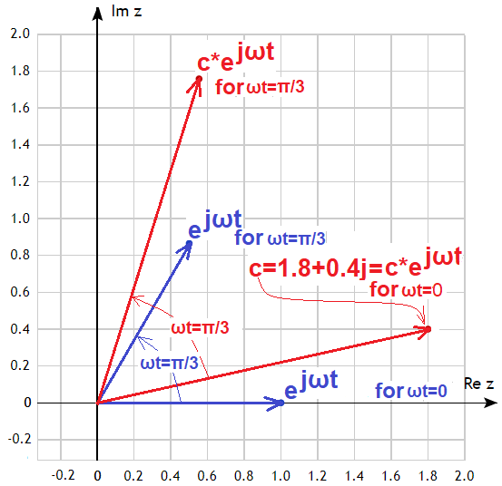

Fig. 3-2
c*exp(jωt) as a rotating vector
We already know that exp(jωt) is a rotating vector of length 1. It is a blue vector in the initial state for ωt=0 and after time t, here e.g. corresponding to ωt=π/3=60º. It is obvious that 2*exp(jωt) will be a vector of length 2, and 3*exp(jωt) of length 3, etc… What about the expression c*exp(jωt), when c is a complex number, e.g.
c=1.8+0.4j? Vector c*exp(jωt) will also rotate. The initial state is just c as c*exp(jωt) for ωt=0, and after a time corresponding to ωt=π/3=60º, the vector will also rotate by 60º as shown in the figure.
Chapter 3.2.2 Components a1cos(1ωt) and b1sin(1ωt) as rotating vectors
Consider the components a1cos(1ωt) and b1sin(1ωt) in Fig. 3-3
They will facilitate the transition from the Trigonometric Fourier Series to the Complex Fourier Series.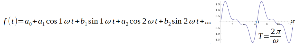

Fig.3-3
The component a0 is a constant and a1,b1,a2,b2… are the cosine/sine amplitudes. The 1ω pulsation corresponds to the period T of f(t). If the parameters a0,a1,b1,a2,b2… are arbitrary then we have the formula for the sum of cosine/sine waves with pulsations 1ω, 2ω, 3ω… and amplitudes a1,a2…b1,b2… If the coefficients are given in Fig’ 2-12 in Chapter 2.2, then f(t) is a Trigonometric Fourier Series. Let’s assume that a1=1 and b1=0.7 and the pulsation, e.g. ω=2.62/sec, was previously measured with a stopwatch. So we are looking for rotating vectors representing the time chart 1cos(2.62t)+0.7sin(2.62t). Vectors can also be treated here as complex numbers.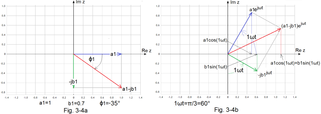

Fig.3-4
a1cos(1ωt)+b1sin(1ωt) as a projection of the sum of rotating vectors (a1-jb1)exp(jωt) to the real axis Re z.
Fig. 3-4a
Rotating vectors in the initial state, i.e. for 1ωt=0. 
a1
-jb1
sum a1-jb1–>see*Note
Fig. 3-4b
Rotating vectors and their sum over time t. Here t is such that 1ωt=π/3=60º.
After time t, the rotating vectors are:
a1*exp(jωt)
-jb1*exp(1jωt)
(a1-jb1)*exp(j1ωt)
The most important conclusion
The expression a1cos(1ωt)+b1sin(1ωt) in Fig 3-1a is the projection of a rotating vecto (a1-jb1)*exp(exp(j1ωt) on the real axis Re z!
Or otherwise
a1cos(1ωt)+b1sin(1ωt) =Re z{ (a1-jb1)*exp(j1ωt)}
The proof of this is the school trigonometry in Fig. 3-4b where the lengths of the rotating vectors blue and green.
are a1=1 and b1=0.7.
The following waveforms correspond to the rotating vectors.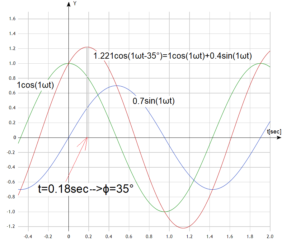

Fig. 3-5
Time charts corresponding to the rotating vectors in Fig. 3-4.
The time chart of 0.7cos(1ωt) is 90° behind 1cos(1ωt) and their sum 1.22cos(1ωt-35°) is behind 35°. Compare with the rotating vectors in Fig. 3-4.
*Note 
This number can also be represented as a modulus |c1|≈1.221 and a phase φ≈-35º or equivalently as Euler 1.221*exp(-j35º).
Modulus 1.221 is Pythagoras with 1 and 0.7 and φ1=arctg(-0.7/1)≈-35º. Check with a calculator.

Chapter 3.3 Complex Fourier Series for 3 harmonics
Chapter 3.3.1 Real axis projection version.
We will start with a Fourier Series in which f(t) has only 3 harmonics. This will be easier:
f(t)=a1cos(1ωt)+b1sin(1ωt)+a2cos(2ωt)+b2sin(2ωt)+a3cos(3ωt)+b3sin(3ωt)
Doubts may arise here.
Firstly
Why break into a Fourier Series a function f(t) which is itself a Fourier Series? The coefficients a0, a1,b1,a2,b2 and a3,b3 can be seen in f(t) and you no longer need to use the formulas in Fig. 2-12 from the previous chapter. Yes, but we do it only for teaching reasons. Anyway, if it bothers you, treat f(t) like any other function and plug it into the formula in Fig. 2-12. You get the same function f(t)!
Secondly
Why are there 6 components here and not 3 as in the title? – Because each single harmonic has a cosine and sine component.
In a specific example, it looks like this:
f(t)=1cos(1ωt)+0.2sin(1ωt)+0.6cos(2ωt)+0.4sin(2ωt)+0.4cos(3ωt)+0.4sin(3ωt)
That is
a1=1 b1=0.2
a2=0.6 b2=0.4
a3=0.4 b3=0.4
Other coefficients a0,a4,b4,a5,b5…=0
The basic pulsation ω can be arbitrary, but if you like to be specific, assume ω=2.6.2/sec as in the animation in Fig. 3-1.
The coefficients c1, c2, c3 can be assigned vectors-complex numbers:
c1=a1-jb1=1-0.2j
c2=a2-jb2=0.6-0.4j
c3=a3-jb3=0.4-0.4j
And the function f(t) rotating vectors-complex numbers
c1*exp(j1ωt)
c2*exp(j2ωt)
c3*exp(j3ωt)
Fig. 3-4 shows:
a1cos(1ωt)+b1sin(1ωt)=Re z {(a1-jb1)*exp(j1ωt)} —>the real part of the rotating vector (a1-jb1)*exp(j1ωt)
Similarly for 2ωt,3ωt
a2cos(2ωt)+b2sin(2ωt)=Re z {(a2-jb2)*exp(j2ωt)}
a3cos(3ωt)+b3sin(3ωt)=Re z {(a3-jb3)*exp(j3ωt)}
So the time function f(t) is the real part of the sum of rotating vectors
c1*exp(j1ωt)+c2*expj2ωt)+c3*exp(j3ωt)
where c1=a1-jb1, c2=a2-jb2, c3=a3-jb3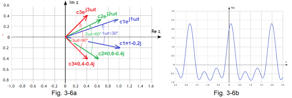

Fig. 3-6
Fig. 3-6a Rotating vectors corresponding to the function f(t)
Fig. 3-6b The function f(t) as the result of the sum of harmonics
c1, c2, c3 are the rotating vectors c1*exp(j1ωt), c2*exp(j2ωt) and c3*exp(j3ωt) in the initial state t=0, and after time t corresponding to the phases 1ωt=30º, 2ωt=60º and 3ωt =90º. It can be seen that after the same time vector c3, which was the most “lagged”, rotated the most. No wonder, since it has the highest rotational speed of 3ωt. Notice that the rotating vectors c1*exp(j1ωt), c2*exp(j2ωt) and c3*exp(j3ωt) at t=0 have the values c1=1-0.2j, c2=0.6-0.4j and c3=0.4-0.4j . It is enough to substitute t=0 into the formulas.
The sum of the projections of rotating vectors on the Re z axis is just a function of f(t)
That is:
f(t)=Re {c1*exp(j1ωt)+c2*exp(j2ωt)+c3*exp(j3ωt)}
Two notess
1. After period T, the rotating vectors will return to their initial state c1,c2,c3. Only vector blue will do 1, green will do 2 and red 3 turns.
2. The c1*exp(j1ωt) + c2*exp(j2ωt) + c3*exp(j3ωt) is a complex periodic function with period T=2π/ω.
3. Rotating vectors resemble a solar system with the Sun at (0,0) and orbits:
c1*exp(j1ωt)–Mars orbit-largest
c2*exp(j2ωt)–Earth orbit
c3*exp(j3ωt)–Venus-smallest
Mars has the lowest angular velocity and Venus the highest, and in this the rotating vectors are similar to planets.
Fig. 3-6 shows the individual rotating vectors, but you can’t see their sum!
The version from Fig. 3-7, in which the sum of the rotating vectors is the end of the vector c3*exp(j3ωt), does not have this disadvantage. This is a more convenient method of adding vectors than the previous “parallelogram” method!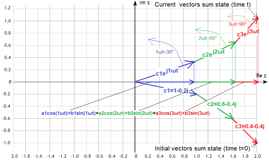

Fig. 3-7
Sum of  rotating vectors c1*exp(j1ωt) + c2*exp(j2ωt) + c3*exp(j3ωt)
The first blue vector rotates around (0,0), green around the blue end, and red around the green end. Subsequent linear speeds are increasing. It’s like the end of a shooting whip breaking the sound barrier.
The lower vector is the initial state at t=0, and the upper one is the state after time t corresponding to the phase 1ωt=30º of the blue vector or, which is the same for the phase 2ωt=60º green and 3ωt=90º red.
After period T when:
–blue will make 1 turn
–green 2 turns
–red 3 turns
will be the initial state again!
Coming back to astronomy this time:
-blue is the Earth orbiting the Sun(0,0)
-green is the Moon orbiting the Earth
-red is an artificial satellite orbiting the Moon.
The rotating vectors c1*exp(j1ωt), c2*exp(j2ωt) and c3*exp(j3ωt) in Fig. 3-7 are accompanied by their projections on the Re z axis, that is:
a1cos(1ωt)+b1sin(1ωt)
a2cos(2ωt)+b2sin(2ωt)
a3cos(3ωt)+b3sin(3ωt)
Therefore, it is obvious that:
f(t)=Re {(a1-jb1)*exp(1jωt)+(a2-jb2)*exp(2jωt)+(a3-jb3)*exp(3jωt)}
That is
f(t)=Re {c1*exp(1jωt)+c2*exp(2jωt)+c3*exp(3jωt)}
Summary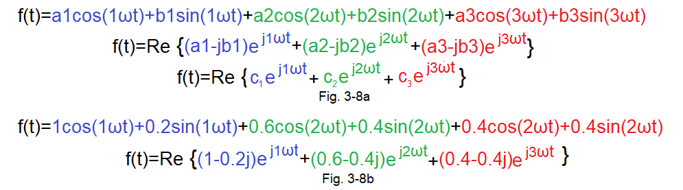

Fig. 3-8
Complex Fourier Series for f(t) with 3 harmonics
Fig. 3-8a
General formula when f(t) has 3 arbitrary harmonics
Fig. 3-8b
Special formula when f(t) has 3 specific harmonics
Chapter 3.3.2 Counter-rotating vector version, otherwise “without Re z” version
Look again at Fig. 3-7. It represents the sum of the rotating vectors c1*exp(j1ωt)+ c2*exp(j2ωt)+c3*exp(j3ωt) and its projection on the Re z axis, here for phase 1ωt=30º. So c1=1-0.2j rotated 30º. This corresponds to the equation in Fig. 3-9a.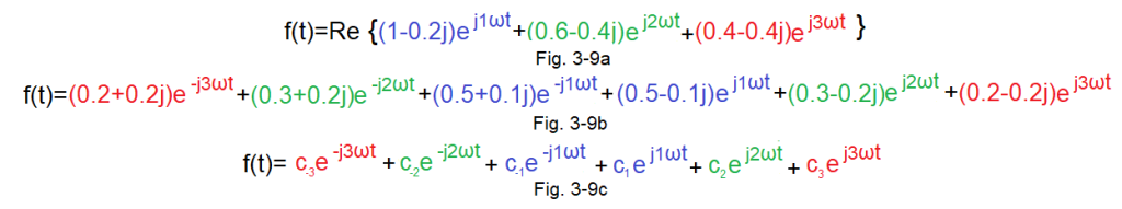

Fig. 3-9
2 equivalent formulas for f(t) with 3 harmonics.
If in the formula Fig.3-9a:
1. We will replace the rotating blue vector
– half of it–>(0.5-0.1j)exp(j1ωt)
– “conjugate half”—> (0.5+0.1j)exp(-j1ωt) which rotates in the opposite direction because it is -j1ωt!
2. We will do the same with the green and red vectors.
This gives us the equivalent formula Fig. 3-9b
Note, that although the new formula is longer, it immediately yields a real number!
Figure 3-9c is a generalization of Fig. 3-9b. Just remember that c1, c2, and c3 are the halves of c1, c2, and c3 in Fig. 3-8a!
I emphasize
Pairs of vectors of the same color are conjugate vectors rotating in opposite directions!!!
The interpretation of the formulas Fig.3-9b and Fig.3-9c is Fig.3-10 with 3 pairs of oppositely rotating conjugate vectors.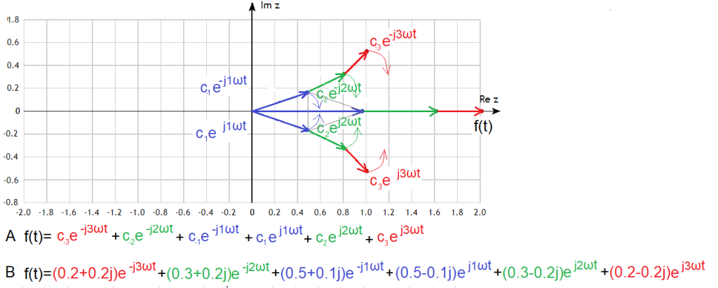

Fig. 3-10
f(t) as the sum of counter-rotating pairs of vectors
A – general formula for any pairs of vectors c(-3), c(-2), c(-1), c(1), c(2) and c(3)
B – special formula for specific pairs of vectors
At first glance you can see that:
1. The bottom rotating vectors are the halves of the bottom rotating vectors in Fig.3-7 for t=0.
2. The upper and lower rotating vectors are conjugate numbers (“mirror image”)
3. The upper and lower vectors rotate in opposite directions and their sum is:
f(t)=a1cos(1ωt)+b1sin(1ωt)+a2cos(2ωt)+ b2sin(2ωt)+a3cos(3ωt)+ b3sin(3ωt)
Explanation for p.3
Formula B is pairs of vectors rotating in opposite directions with complex coefficients c(-1), c1, c(-2),c2 and c(-3),c3 “photographed” in Fig. 3-10 at time t=0.
For example, the pair (0.5-j0.1)exp(j1ωt) and (0.5+j0.1)exp(-j1ωt) gives the sum = the blue vector on the Re z axis. It is equal to the blue horizontal vector on the Re z axis in Fig. 3-10 is 1cos(1ωt)+0.2sin(1ωt). This vector will move according to this formula only along the Re z axis.
It is analogous with the rotating pair of green and red.
The sum of all the rotating vectors will give us a particular pattern B and a general pattern A.

Chapter 3.4 Complex Fourier Series – general formula with real part
Chapter 3.4.1 Basics
And now the most important
1. Take any periodic function f(t) with period T
2. Calculate the fundamental pulsation ω=2π/T
3. Calculate the coefficients a0,a1,b1,a2,b2,…an,bn… and then the real coefficient c0 and the complex coefficient c1,c2,c3…cn…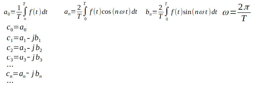

Fig. 3-11
Formulas for Fourier coefficients
Now we can determine the final general formula for the Complex Fourier Series with a real part.
We can now find the final general formula for a Complex Fourier Series with a real part.

Fig. 3-12
The formula is a generalization of Fig. 3-8a. The constant component c0 appeared. Not very visible because of the yellow color. It accurately approximates the function f(t) only for n=∞, but practically a dozen, maybe a little more, of the first components is enough.
Each component c1*exp(1ωt), c2*exp(2ωt), c3*exp(3ωt),c4*exp(4ωt)… c∞*exp(∞ωt), is a rotating vector as in Fig. 3-13.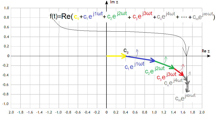

Fig.3-13
The yellow vector c0 is a constant component and is the only one that does not rotate. Or formally it rotates, but with a pulsation ω=0. The others rotate faster and faster “each around the previous end”, i.e. indirectly around the fixed end c0. Successive vectors are getting shorter and shorter, and the last c∞ is usually of zero length and rotates infinitely fast! The closer to c∞, the polyline in Fig.3-13 approaches the continuos line! The projection of the end of the last vector on the real axis is just our periodic function f(t). Try to imagine these rotating vectors. Doesn’t it remind you of the end of the shooting whip?
In other words
The vectors are rotating and the projection of endpoint c∞ on the real axis moves exactly like the function f(t)!
Just as there are no ideals in life, the last rotating vector is e.g. c20*exp(j20ωt) and not c∞*exp(j∞t). This is quite enough to approximate the f(t) function as accurately as possible.
Note:
The “last” rotating c∞*exp(j∞t) usually has a length of zero. But the sum of all rotating vectors, the point c∞*exp(j∞t) points to, has a finite value You will find out in a moment!
Chapter 3.4.2 Example with a square wave
Nothing appeals to the imagination like a specific example, e.g. with a square wave. It is discussed in detail in chapters 2.5 and 2.6 as a trigonometric series.
Go back there for a while. A square wave with a pulsation of ω=2π (i.e. T=1sec) is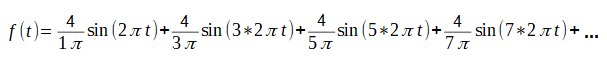

Fig. 3-14
Trigonometric Series of a square wave with ω=2π/sec.
Note, that the constant component c0=0, which is obvious and
c2=c4=…=c2n=0 because the square wave f(t) in Fig. 2-13 is an odd function. Also the “cosine” coefficients are zero b1=b2=b3=0….
From the sine/cosine coefficients in Fig. 3-14 and the formulas in Fig. 3-11, it follows directly that:
c1=-4j/π, c3=-4j/3π, c5=-4j/5π, c7=-4j/7π
and The Fourier Trigonometric Series of a square wave can also be represented as a Complex Fourier Series.
Notice that you didn’t even have to calculate the integrals. But if you insisted, because you like 2 mushrooms in borscht, then substituting f(t) from Fig. 3-14 into the formula of Fig. 3-11, the result would be identical.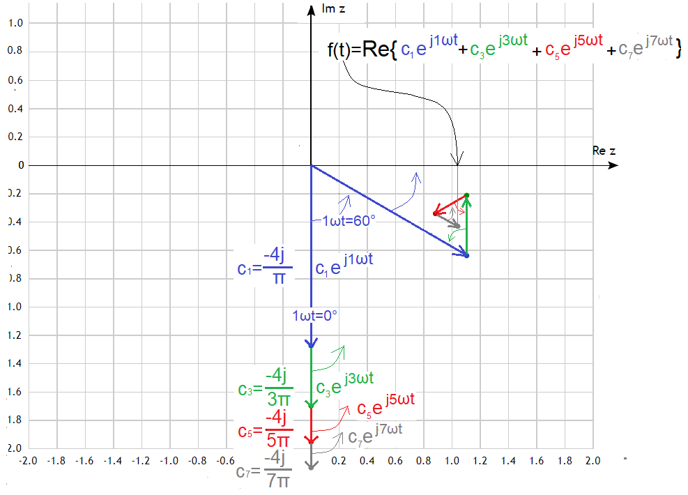

Fig. 3-15
Complex Fourier Series of a square wave
The initial state, i.e. for t=0, are successive vertical vectors on the lower imaginary semi-axis Re z. Only the first 4 are visible, as c1, c3, c5 and c7. The “even” vectors c0,c2,c4,c6…as stated earlier, are zero. The last c∞, although its length is zero, lies at infinity on the negative “end” of the imaginary axis Im z. Here read the concluding remark of the previous section.
I also showed the state of the vectors when c1 rotated by 1ωt=60º, c3 by 3ωt=180º, c5 by 5ωt=300º, and c7 by 7ωt=420º. Evidently, the vector c7exp(7jωt) was the fastest to make the largest rotation (420º i.e. full rotation + 60º), especially compared to the slowest c1exp(1jωt). And how to read f(t) as a sum of rotating vectors? Here you go, for t=0 it is a projection on the Re z axis, i.e. f(0)=0, and for t corresponding to a rotation of 1ωt=60º=π/6 it is also approximately the projection of the end of the vector c7exp(7jωt) on Re z.
Why roughly? Because I haven’t yet considered the remaining vectors c9exp(9jωt)…c∞exp(∞jωt) ending at the finite point c∞. This point is somewhere near the end of the vector c7exp(7jωt) and you have to visualize it somehow. Only the projection of this vector produces a perfect square wave.
Let’s consider the graph in Fig. 3-16 again. For simplicity, let’s assume that our function f(t) has only 3 first harmonics, i.e. only 3 vectors c1, c3, c5 will rotate with velocities 1ωt, 3ωt and 5ωt.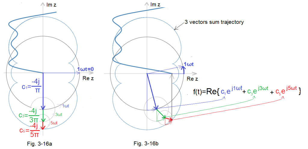

Fig. 3-16
Fig. 3-16a Initial state for phase 1ωt=0.
Fig. 3-16b State for 1ωt phase. The vector c5exp(j5ωt) rotates around the c3exp(j3ωt) end, which in turn spins around the c1exp(j1ωt) end. This resembles a system with the Sun at (0,0), the Earth revolving around the Sun, the Moon around the Earth, and the Satellite around the Moon. After a time corresponding to 1ωt=2π, the initial state will again be as in Fig. 3-16a, except that “Earth” will make 1, “Moon” 2 and “Satellite” 3 rotations.
The projection of the “Satellite” on the Re z axis follows the formula { c1exp(j1ωt)+c3exp(j3ωt)+c5exp(j5ωt)}.
These are the first 3 “non-zero” harmonics of the decomposition of a square wave into a Trigonometric Fourier Series.
The expression c1exp(j1ωt)+c3exp(j3ωt)+c5exp(j5ωt)  alone are the first 3 components of the Complex Fourier Series of a square wave.
Note that the path of the Satellite around the Sun (and not around the Moon) is no longer a circle but some strange contortion! It turns out that with the right combination of complex coefficients cn and a large n, the satellite will rotate along any path. Even square! So, given the appropriate cn, we can draw any images. This is what the theory of image processing has been dealing with recently. Fourier must be turning over in his grave.
Note
The circle in Fig. 3-1 is a function that assigns to each time t a corresponding point z=1exp(jωt) in the plane of complex numbers z.
By analogy
The path of the sum of 3 vectors in Fig. 3-16 is a function that assigns to each time t a corresponding point z=c1exp(j1ωt)+c3exp(j3ωt)+c5exp(j5ωt) in the plane of complex numbers z.

Chapter 3.4.3 Animation (from youtube)
Click on YouTube’s „play” triangle. GLV author’s nickname.

Fig. 3-17
Animation of a Complex Fourier Series of a square wave
The spinning upper 4 vectors are the 4 components of the formulaf(t)=Re{c0+c1exp(j1ωt)+c3exp(j3ωt)+c5exp(j5ωt)+c7exp(j7ωt)}Successive harmonics with decreasing amplitudes and increasing pulsations of 1ωt, 3ωt, 5ωt and 7ωt are perfectly presented. They are vector sums and sine sums. Of course, both give the same result, which is a function of time f(t) close to a square wave.

Chapter 3.5 Complex Fourier Series – general formula without real part
And now the most important thing, the second tadam!!!
1. If you take any periodic function f(t) with period T
2. Calculate the fundamental pulsation ω=2π/T
3. Calculate the coefficients a0,a1,b1,a2,b2,…an,bn… and then the complex coefficients
…c(-n)…c(-3),c(-2),c(-1),c0,c1,c2,c3…cn… acc. formulas Fig. 3-18
then
you will get the formula Complex Fourier Series–>Fig.3-19
Note for the above designations. e.g. c(-3) is c with negative subscript -3. I can’t save the subscript in WordPress.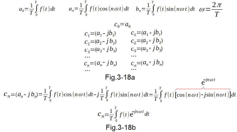

Fig. 3-18a
The formula for the complex coefficients c(n) of the Complex Fourier Series “without real part”
Fig. 3-18b
The same formula for c(n) after taking into account Euler’s formula exp(jωt)=cos(ωt)+jsin(ωt)
Compared to formula Fig. 3-11
1. c0, i.e. the constant component coefficient is identical
2. The other coefficients cn are the complex numbers and halves of Fig. 3-11 (because an and bn are the halves of an and bn of Fig. 3-11)
3. The pairs c(n) and c(-n) are conjugate numbers. So their sum c(n)+c(-n)=2a(n) is a real number.

Fig. 3-19
Formula for Complex Fourier Series
Negative pulsations and coefficients with negative indexes appeared. There are now 2 times more* of them with 2 times smaller modulus, but they all add up to the same real function f(t)!
*compared to Fig. 3-11

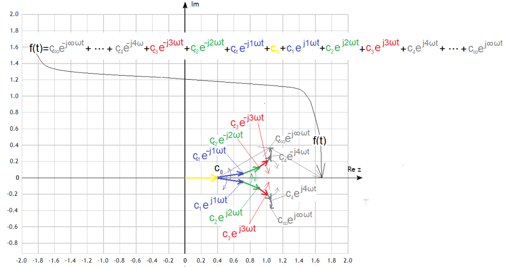
Fig. 3-20
Complex Fourier Series as a sum of counter-rotating vectors
More precisely, “Sum of counter-rotating vectors + constant component c0“
The justification is very simple:
Each pair of oppositely rotating vectors is, for example:
c(3)exp(j3ωt)+c(-3)exp(-j3ωt)=a(3)cos(3ωt)+ b(3)sin(3ωt). This is explained in detail in Chapter 3.3.2.
So the sum of all pairs + the constant component c0=a0
will give us the formula Fig. 3-3
That is the formula Fig. 3-19
In an elegant and condensed form, it looks like this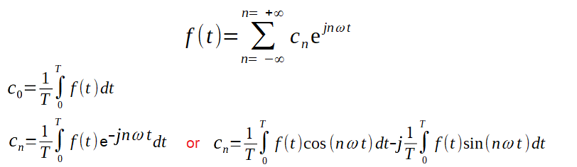

Fig. 3-21
Complex Fourier Series
The “no real part” formula is more common than the equivalent “real part” version.
Therefore, it is simply the formula for the Complex Fourier Series.
By the way, you learned that there is such a thing as positive and negative frequency/pulsation. Positive have sinusoids whose vectors rotate counter-clockwise, negative – clockwise. It used to intrigue me. One can somehow imagine that the zero frequency is DC (direct current). But negative? Something more “solid than solid”? And how to live here? Now I know.