29. Disturbances Analysis - How does it work?/Jak to dziala?

Automatics

Chapter 29 Disturbances analysis
Chapter 29.1 Introduction
Automatics has 2 main tasks:
1. Getting the output signal y(t) to the setpoint x(t) by a man – operator of the technological process.
The ideal is a steady state where x(t)=y(t). This should also be a “nice” response to the unit step x(t). What “pretty” or “optimal” means is another matter.
For the first, this will be the shortest regulation time, even with oscillations.
For the second one, also the shortest time, but without oscillations.
The third one already allows 10% oscillation.
The First, Second and Third is Mr. Technologist or Mr. Customer who gives automatics engineer to earn. Most of the experiments in this course are the study of the response of y(t) to unit step x(t).
2. Ensuring disturbances suppression z(t).
They are constantly trying to push the output y(t) out of the virtue path of keeping y(t) at the set point x(t). This is what the controller fights against. The ideal is a state where, despite the disturbances, e(t)=0 is still present. This is only possible in theory. In practice, it is only after some time that the disturbance z(t) will be completely suppressed. You found out about it by examining the influence of z(t) disturbances in I, PI and PID control. Although the P and PD control suppresses the error, it does not completely. It only reduces it to, for example, 2%, compared to the system without control.
Note
An optimal step response x(t) generally does not provide an optimal response to a disturbance z(t) and vice versa.

Chapter 29.2 Effect of setpoint x(t) and disturbance z(t) on output signal y(t)
– The action of x(t) on y(t) is contained in the transmittance of the closed system Gz(s)=y(s)/x(s)
– The action z(t) on y(t) is included in the disturbance transmittance Gzakl(s)=y(s)/z(s)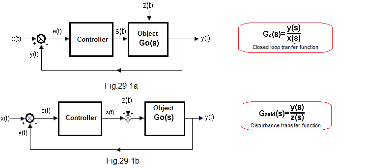

Fig. 29-1
Fig. 29-1a is used when we do not know exactly what the impact of disturbances z(t) on the object is. We feel that the controller is trying to suppress the disturbance, but how it does it is up to it. In this form, it is impossible to check how y(t) will respond to the disturbance step z(t). Therefore, a more accurate will be Fig. 32-1b with a specific situation. Here, the disturbance z(t) is added directly to the control signal from the controller s(t). For example, when the object is a furnace and s(t) is the power supplied from the controller to the heater. The positive interference z(t) will then be the power supplied to a separate heater located close to the control heater.
Let’s introduce some more math. Here R(s) is the transmittance, which can be a PID controller.

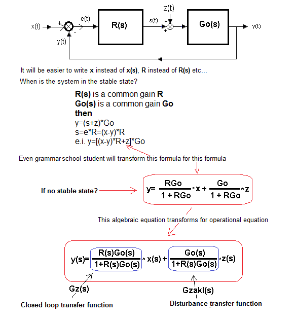
Fig. 29-2
Note that the transmittance of a closed system Gz(s) is the same as “in the most important formula”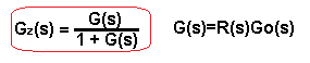

Fig. 29-3
On the other hand, there is no R(s) in the disturbance transmittance nominator Gzakl(s). So Gzakl(s) has a little less inertia than Gz(s). Therefore, the response to z(t) is usually a bit faster than x(t)! Therefore, when we choose the PID settings, we must make a decision.
What do we care more about?
On the optimal response to x(t) or z(t)?
If changes of the setpoint x(t) occur frequently, we tune the controller due to the setpoint x(t), if rarely, due to z(t). More often, however, we are guided by tuning the controller due to the setpoint x(t), because it is more predictable than the disturbance z(t). It’s like the method of the guy who looks for the key under the lamppost just because he can see better. On the other hand, tuning differences due to x(t) or z(t) are rarely shockingly large.
And when the disturbance is in the “center” of the Go(s) object, as in Fig. 29-4a?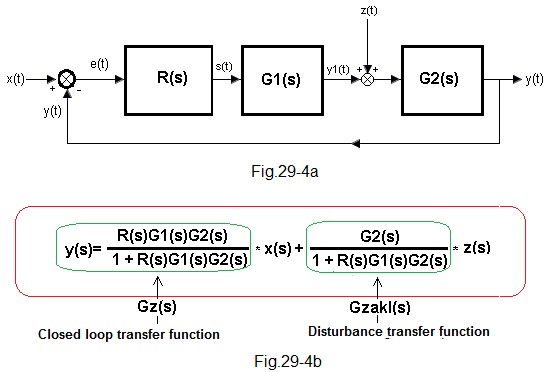

Fig. 29-4
Fig. 29-4a is a more accurate approximation Fig. 29-1a, in which z(t) appears in the “middle” of the object Go(s)=G1(s)*G2(s), i.e. between the transmittances G1(s) and G2(s).
The formula in Fig. 29-4b results directly from Fig. 29-2. It is enough to assume that G1(s) is part of the transmittance of the controller and is R(s)*G1(s) and the object will be G2(s). The formula for the disturbance transmittance Gzakl(s) shows that the closer the disturbance z(t) is to the exit of the object, the more pronounced will be its impact on y(t). What does “closer to the exit” mean? The fact that the G2(s) inertia is lower compared to the G1(s) inertia. Otherwise, the transmittance G2(s) becomes closer to the proportional term G2(s)=1. So the disturbance z(t) will be less “flattened” by G2(s). You will find out later in this chapter.

Chapter 29.3 Two-stage heat exchanger
Chapter 29.3.1 Why do we visit the thermal engineering?
Two-stage heat exchanger is a good analysis example for:
– Disturbance analysis
– Different control systems structure –>useful in the next chapter
Chapter 29.3.2 Two-stage heat exchanger as a opened loop
We will examine the object itself without control, i.e. in an open system.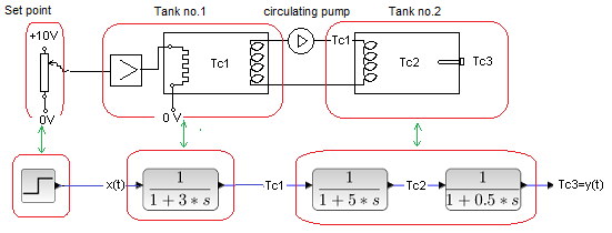

Fig. 29-5
The scheme is to be used to learn the principles of automatics, not the thermal processes occurring in the exchanger. That is why we will make very large simplifications.
1– The liquid does not evaporate or freeze. So it can reach a temperature of e.g. +1000ºC or even –1000ºC, which is even more absurd. A heating plus on the heater is normal, but a cooling minus? However, since the 19th century, the so-called the Peltier element. Such a heater-cooler makes it easier to understand the negative sPID(t) control signal, which in some very short moments “wants” to cool the liquid to a temperature of e.g. -1200 ºC!. What does “wants” mean? That it won’t cool down to that temperature right now. But if such a cooling power (i.e. negative) was fed to the heater-cooler all the time, then after some time the liquid would reach -1200 ºC.
2- In the tanks, the mixers are constantly working (they are not shown in the diagram), i.e. in every place of a given tank there is the same temporary temperature Tc1 or Tc2. Instantaneous Tc1 may differ from instantaneous Tc2. It can increase or decrease depending on the position of the potentiometer slider.
3– Heat is transferred from tank No. 1 to tank No. 2 through the output coil of the tank. 1 and inpput coil of the tank. 2. Heat transport is facilitated by a circulation pump, similarly to a pump in a building that forces water to flow through radiators. The liquid in the input coil of tank No. 2 has a temperature of Tc1, i.e. the temperature of the liquid in tank No. 1. Therefore, Tc1 is the input signal to tank No. 2. Similarly, the voltage from the amplifier to the heater is the input signal for tank No. 1. In steady state, Tc1 = Tc2 =Tc3.
4-The power on the heater is proportional to the voltage from the amplifier, not the square of the voltage. This, of course, is contrary to electrical engineering, but thanks to this, the temperature of the liquid will be proportional to the voltage from the adjuster and it will be easier to analyze the waveforms.
5- If there is e.g. +10V on the setting unit, corresponding to the temperature of +100ºC, then after some time in the tank No. 1 will show Tc1=+100 ºC and then in tank. No. 2 will also be Tc2=+100 ºC. This temperature “covering” the housing of the platinum sensor (platinum wire) will heat the wire and the transmitter will show the temperature Tc3=+100ºC in the form of +10V voltage.
Note that in steady state the input is +10V and the output is +10V. So the whole exchanger with the power amplifier, coils, etc. can be treated as an amplifier with a gain of K=1 and a certain dynamics -> here a three-inertial term. It makes the analysis so much easier!
Similarly:
+5V–>Tc1=Tc2=Tc3=+50ºC–>+5V
0V–>Tc1=Tc2=Tc3=0ºC–>0V
-5V–>Tc1=Tc2=Tc3=-50ºC–>-5V
-10V–>Tc1=Tc2=Tc3=-100ºC–>-10V
6– Zero initial conditions–> Tc1=Tc2=Tc3=0ºC
7 – A power amplifier with a voltage gain of ku=1 ensures that there is a voltage x(t) across the heater regardless of the load (or resistance) of the heater.
We will examine the influence of the location of the disturbance on the output signal y(t). It turns out that the closer the disturbance z(t) is to the exit of the object, the more pronounced its influence. The disturbance z(t) will enter the three-inertial object Go(s), an example of which is a heat exchanger.
The slider of the setpoint x(t) in Fig. 29-5 will now be rapidly moved from the middle position to the upper position. In this way, you will step the temperature from x(t)=0ºC to x(t)=+100ºC. This corresponds to the model and animation.

Fig.29-6
A step of 0ºC to +100ºC which corresponds to a step of 0 to 1
Model of the exchanger in the previous drawing. There is no power amplifier in it because ku=1.
Given the small time constants, our tanks are the size of glasses. Therefore, a decent amplifier-emitter follower should be enough to control the heater. Here part of the power is lost in the transistor. For larger exchangers, pulse amplifiers are used. Let’s not delve too much into whether there are such small Pt100 thermometers in the housing. Suppose there are such midgets.
The three-inertial nature of the signal Tc3=y(t) is clearly visible and how the temperature Tc1 leads Tc2, and Tc3. Due to the small time constant of the thermometer, Tc3 is almost Tc2.
Our assumptions were confirmed that:
– instantaneous temperatures Tc1, Tc2 and Tc3 may be different
-in steady state all temperatures are equal->Tc1=Tc2=Tc3=100ºC
Chapter 29.3.3 Exchanger in a closed system
Classic automatic control system without disturbances.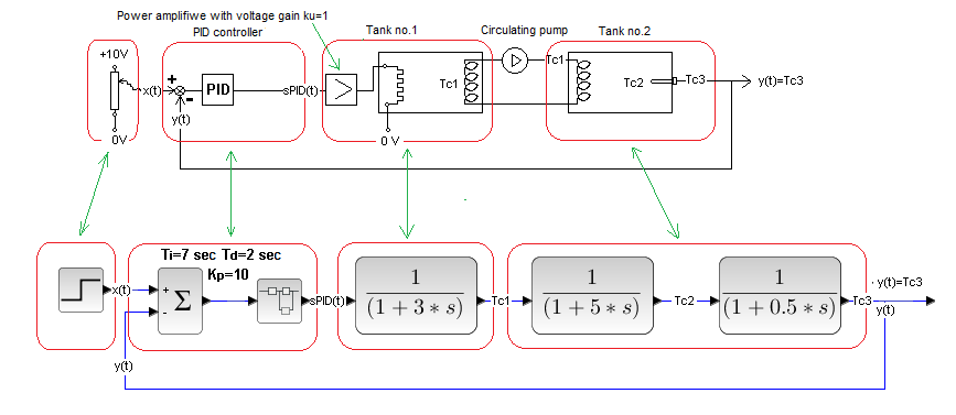

Fig. 29-7
The flowchart at the top and the corresponding block diagram at the bottom.
The input to the tank 1 is the signal from the PID controller, and more precisely from its power amplifier, and the output is the temperature Tc1 of the output coil, the same as the temperature of the liquid in the tank 1. It is also an input signal to tank 2, because in its coil there is also temperature Tc1.

Fig. 29-8
If you look closely, you have already studied this diagram–>Chapter 27 Fig.27-29. Then only you did not associate it with 2 heat exchangers and with the voltage output Tc3 0 … + 10V on the Pt100 thermometer. Actually, on its converter, which converts changes in the resistance of a platinum wire (hence the name PT100) into voltage changes.
General note
There are a lot of time charts here, from which you can get nystagmus. To make the task easier, I suggest analyzing it “piece by piece”.
1. First, the most important, i.e. input and output, i.e. x(t) and y(t).
2. Error e(t)=x(t)-y(t)–>Check if it is true for each t.
3. SPID(t) control signal. Or would you do it manually?
4. The next “softening” signals Tc1, Tc2 and Tc3. Note that you have already analyzed Tc3 as y(t)=Tc3.
Apply this rule later as well.

Fig. 29-9
The previous time chart just a different oscilloscope scale, so you also see what was “crop” in Fig. 29-8.
The setpoint x(t) forces a step in 3 sec. +10V. So it “wants” that after some time the thermometer will also be +10V. So y=Tc3=+100ºC. We remember that the initial temperature of the liquid in the tanks Tc1=Tc2=0ºC. In 3 seconds (at the moment of jump) error e(t)=+100ºC. The P component of the PID controller then forces the control signal corresponding to the power which in steady state (if it did not change) gives +1000ºC! (here Tc1=10) Shock? It could be even bigger. After all, the D component differentiates the jump and gives =+200 . In total, at the moment of the jump, the controller gives the signal sPID(t)=210, which corresponds to the temperature of +21,000ºC. More than in the sun! And so we are lucky that in the PID controller the differentiating component D is real, i.e. “flattened” by the inertial unit. If it were a perfect differentiator, then the power on the heater would correspond to an infinite temperature for a while! The hydrogen bomb is a piece of cake. And all this happens in tank 1 smaller than a glass.
Why am I scaring my readers? To be aware that so far we have modeled ideal objects. There were no restrictions. And in life, and even more so in electronics, they occur. Our power amplifier – the emitter follower enters the saturation resulting from its power supply, e.g. -15V…+15V. In ideal systems, negative voltage cools with temperature. In real systems, a negative SPID(t) signal only turns off power to the heater. So the temperature Tc3 will drop only to the ambient temperature. And besides, even in ideal systems there are no “hydrogen bombs” – powerful energies. So what if there are very high powers for very short moments. But energy can be normal now because it is power*time.
By the way. Control systems with a Peltier element are used only in special cases, when very fast temperature changes are required.
What is the conclusion? Ideal time charts give very strong control signals for very short periods. At the beginning of the jump x(t) the control signal sPID(t)=210 which corresponds to the temperature of +21000ºC! The temperature of the liquid, of course, does not have time to reach this value, but it increases very quickly. Feedback reduces this signal even faster, even for a moment it wants to cool the liquid to -1200ºC! This can be seen in Fig. 29-9. Real runs have limitations and will therefore be slower. In addition, the setpoint x(t) is changed rather rarely. Most often, the regulator works in the disturbances suppression mode z(t) and not when the setpoint x(t) changes. Disturbances z(t) are usually much smaller than spikes x(t). Then the control signals sPID(t) are less saturated and the waveforms will be closer to ideal. You will learn more about this in chapter 31.

Chapter 29.4 Exchanger temperature control with disturbances in different places
Chap. 29.4.1 Introduction
Fig. 29-4b shows that the closer the disturbance z(t) is to the output y(t), the stronger its influence will be. We will check it in our exchanger. We will introduce a disturbance z(t) before the first, second or third inertia on the control system in Fig. 29-7. The disturbance will be the insertion of an additional heater. We’ll see how the PID controller handles it. Finally, we will introduce the most malicious disturbance – directly to the output of the thermometer.
Chapter 29.4.2 Disturbance before first inertia – auxiliary heater at tank heater 1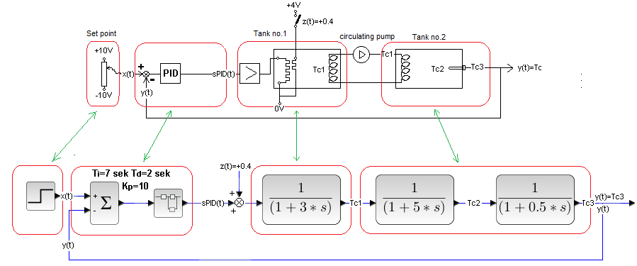

Fig. 29-10
The disturbance will be a +4V voltage step (contact short) on the additional heater right next to the main heater in tank 1. This will cause additional heating. The resistances of the heater controlled by the amplifier and the additional heater are the same. That is, the same voltage across the two heaters causes the same increase in the temperature of the surrounding liquid.

Fig. 29-11
In steady state, the disturbance z(t) caused by 40% heating was compensated by the PID with a voltage drop (cooling) of 40%. As a result, the temperature y(t) barely moved. Let me remind you that 1 on the chart corresponds to the temperature +100ºC.
Chapter 29.4.3 Disturbance before secondinertia – additional heater at Tank 2 coil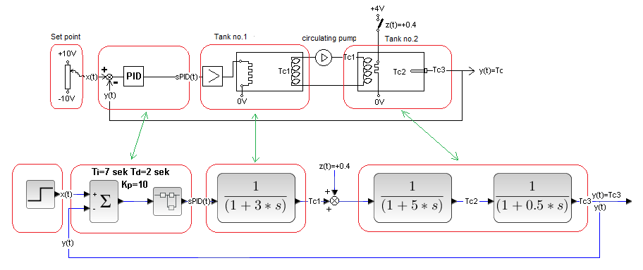

Fig.29-12

Fig. 29-13
The response of y(t) to the setpoint x(t) is the same as before. It is obvious
The reaction y(t) to the disturbance z(t) is more rapid and shorter than before. The reaction of the PID, i.e. the blue sPID(t), is also stronger.
Chap. 29.4.4 Disturbance before the third inertia – the heater acts directly on the thermometer part of the tank No. 2
You will see how malicious a disturbance acting directly on the output or very close to the output can be. The disturbance z(t) is the voltage step on the heater, which is a resistance wire wound on the housing of the Pt100 thermometer.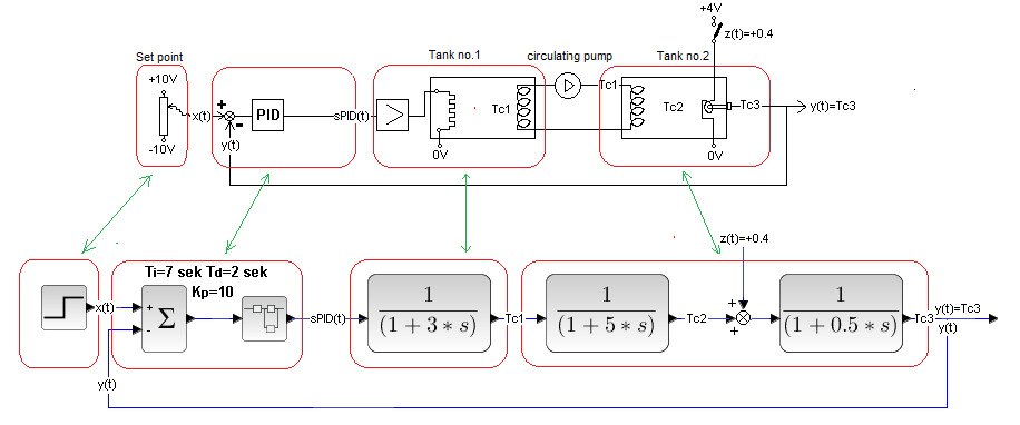

Fig. 29-14
Several turns of the resistance wire of the heater “circle” a piece of the thermometer housing.
Therefore, the thermometer is affected by:
– liquid temperature Tc2 in tank 2
– a heater “circling” a piece of thermometer
We also assume that the parameters “heating the thermometer” from the heater are the same as the parameters “heating the thermometer” from the liquid flowing around the part of the thermometer not covered by the heater.
The disturbance will be a voltage jump z(t)=+4V on the heater.

Fig. 29-15
In steady state, the disturbance z(t) caused by the 40% additional heating of the thermometer was compensated by the PID with a 40% power drop. The disurbance effect is even stronger than before because the disurbance is closer to the PID input. Therefore, the controller reacts more vigorously to z(t). This is visible in the blue sPID(t). We’re glad it’s okay. Tc3 has returned to its previous value. But what is Tc3? This is the voltage on the thermometer. And for us, the temperature of the liquid Tc2 in the second tank is important, not some voltage. Let’s examine the time chart of Tc2.

Fig. 29-16
Contrary to the previous diagram, we can also observe the temperature of the liquid Tc2 in tank 2. The real temperature of the liquid is Tc2. Note– Tc2 is yellow and this color is barely visible on a white background! It turns out that in steady state, the liquid in tank 2 has Tc2=60ºC! Simply, PID, like any decent controller, tries to equate the output signal y(t)=Tc3 with the set value x(t) corresponding to the temperature of 100ºC. And he succeeds 100% of it, as you can see in the red y(t). It’s just that the thermometer readings are falsified by additional heating of the thermometer housing. The controller “thinks” that the temperature of the liquid is Tc3=100ºC. Meanwhile, in steady state Tc3=Tc2+40ºC=100ºC. So Tc2=60ºC as you can see in the attached picture.
There were specific mining accidents. A methane sensor was specially blown with fresh air. The methane concentration at the sensor itself was fine and machines with sparking electric motors were not shut down. There was a mining bonus and 100 times the Russian roulette was successful, but the 101st time … The measurement result was falsified, just like in our example with heating the thermometer housing.
Chapter 29.4.5 Most Malicious Disturbance – Direct to Output! (behind the thermometer)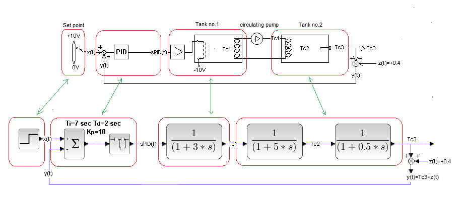

Fig. 29-17
This is a similar disturbance to the previous one, but more venomous. Here we do not heat the thermometer, but we add voltage to the thermometer output! That is total fraud. The controller receives a “false” high temperature y(t)=Tc3 + z(t). In a steady state, the regulator will do its job, i.e. it will equal x(t)=y(t), but the real temperature of the liquid will be equal to Tc3(t)=y(t)-z(t)=100ºC-40ºC=60ºC.

Fig. 29-18
When z(t)=+0.4 appears in 25 seconds, the controller thinks that there is now y(t)=+140ºC in the tank (although Tc3=+100ºC). Therefore, trying to bring the error e(t) to zero, it will reduce the heating, i.e. sPID(t), so that y(t) is 100ºC again. And he will succeed only that then the steady state will be Tc3=+60ºC.
Compare the response of y(t) to a disturbance with Fig. 29-16. Here the jump y(t) to 1.4 (i.e. to +140ºC). Why. Because here the voltage is added to the thermometer, and in Fig. 29-16 the thermometer was heated.

Chapter 29.5 Key Disturbances Conclusions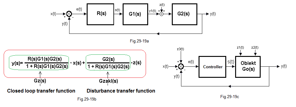

Fig. 29-19
1. The closer to the output, the more pronounced the impact of the disturbance.
According to Fig. 29-19c, the disturbance z2(t), which is “closer” to the output y(t), will cause a stronger control signal s(t) and more pronounced changes in y(t) than the disturbance z1(t).
The justification is the formula in Fig. 29-19b showing the relationship between the disturbance z(t) and the input x(t) and the output y(t). The more z(t) moves to the right to output y(t), the more the inertia of G2(s) decreases. And what does that mean? The “inertia” of the disturbance transmittance Gzakl(s) decreases because its nominator tends to 1. So the response z(t) is clearer and shorter. This is confirmed by the time charts y(t) in Fig. 29-11, 29-13, 29-15, 29-16 and 29-18, where z(t) “moves” from left to right.
2. Disturbance directly to the output – the most perfidious
An example is the sensor in chapter 29.4.4 and 29.4.5. It gives the controller false information, to which the controller reacts as if it were true. This is not only in automatics. The most malicious are disturbances, i.e. falsified signals that directly affect the decision-making process. Have you read “The Needle” by Ken Follett? Here British intelligence tipped Hitler’s best agent (that is, Hitler’s sensor) the information that the 1944 invasion would be here, and not there. And Adolf stopped his best divisions for a few days.
A direct disturbance to the output is also a disturbance to the input (with a changed sign). Another example is z(t) in Fig. 29-18. The controller “thinks” that the setpoint is x(t)+z(t) and tries to adjust the value of y(t) to it. It’s as if spy disguised himself as Hitler and gave orders. That is why engineers try to protect the tiny controller against distuurbances as much as possible. And this is easier than securing the entire control system, especially the big industrial facility.