Automatics
Chapter 28 PID controllers tuning
Chapter 28.1 Introduction
In chapters 23..27 we discussed the principle of operation of the P, PD, I, PI and PID controllers. I think that by manually selecting Kp, Ti and Td settings by trial and error method, you understood their roles well. By the way, you learned the first method of setting settings. Trial and error method, also used in other fields far from automatics.
Example
You are very careful when skiing for the first time. You make big bends, you brake for a long time, you fall over. You are similar a PID controller with very careful settings. Small Kp and Td, there is almost no integration, i.e. very large Ti. As you learn, you gain experience, the movements are more and more precise. And what does this mean in the language of automatics? The fact that you improve the settings of your private controller Kp, Ti, Td encoded in your brain. After all, you are slalom between the poles. Your controller is now almost optimal. I suspect that Swiątek, Williams or another Djokovic, the best tennis players in the world, have settings of their regulators very similar to each other. But only the champion has a little better. I’m done with this naive and greatly simplified philosophy.
What did it stand for? That the first approach to tuning controllers (i.e. matching Kp, Ti and Td) is the trial and error method –> otherwise, the manual method. Now let’s move on to the serious methods.
I will present some old-fashioned methods invented during World War II by a certain Ziegler and Nichols:
– Step response method
– Self oscillation method
Each is an example of a different school. The first requires a mathematical description, i.e. the Go(s) transmittance of the object. The second is only to examine the object, and more precisely, to measure the period of oscillations with some gains of the so-called critical. So she is less fussy about the exact knowledge of the object.
Chapter 28.2 Step response method
Chapter 28.2.1 Introduction
Requires knowledge of the mathematical model of the object.
We can get the model by:
– accurate mathematical analysis through knowledge of physical and chemical processes. This is of course a task for the ambitious.
– We do not go into any thermodynamics, we only study the response to a unit step x(t). The task is less ambitious and easier, so we will discuss it.
There will be 4 stages in it.
1-Studying the object’s response to a step x(t) in an open system and determining the approximate transmittance Gp(s) as inertia T and delay To
2-Determination from the appropriate tables of optimal settings Kp, Ti and Td
3-Checking the response to a closed system step
4-Trying to find better settings manually
Chapter 28.2.2 Step 1 – Examining of the object’s response to a step in an open system
Fig. 28-1
This is a typical multi-inertial unit, here four-inertial
On a real object, of course, you don’t know this transmittance. You only guess that it is a multi-inertial unit. What is this “multi“, what are the time constants T1,T2,T3 and T4? You do not know that. I will only add that many processes, especially in the chemical industry, are of this nature. Focus on the black step x(t) and the red response y(t). You see the characteristic elbow, or inflection point. A tangent was drawn through this point and the parameters K, T and To of the equivalent transmittance Gp(s) were determined from this construction. This topic has been discussed in detail in chapter 10 Fig. 10-5.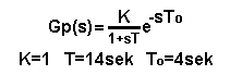
Fig.28-2
Determined object parameters K, T and To.
Chapter 28.2.3 Step 2 – Determination from the appropriate tables of optimal settings Kp, Ti and Td
According to Mr. Ziegler, there are several optimal combinations of Kp, Ti, Td for the same step x(t) response. how is it? After all, the optimal set of Kp, Ti and Td. There can only be one winner. Holy truth, but the first optimum is for the shortest time without overshoots. The second is also the shortest time, but e.g. with 20% overshoot, and the third is the criterion for the minimum integral of the square of the error. The very name of the third arouses reluctance. Therefore, we will tune the controller according to criterion No. 2, and it says this:
For the PID controller and the object from Fig. 28-3, the following settings of the PID controller will ensure the shortest control time with an overshoot of no more than 20%.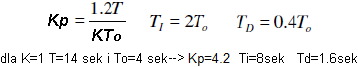
Fig. 28-3
Formulas and calculated settings for an object with parameters from Fig. 28-2. There are some limitations. Namely, the To delay It must be in the range of 0.15T…0.6T. So, for example, pure inertia or pure delay is out. The condition is obviously met because 2.1 sec<4 sec<8.4 sec. So let’s check what the response to a step x(t) looks like with the above settings.
Chapter 28.2.4 Step 3 – Closed loop response checking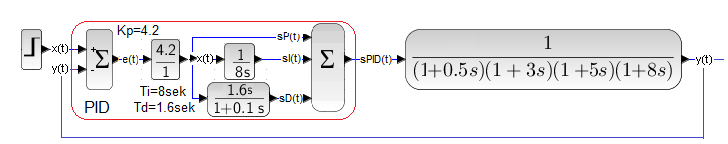
Fig. 28-4
Closed system with optimal settings from Fig. 28-3.
Fig. 28-5
What would I say here? First of all, the overshoot is 50%, not 20%. Secondly, the control time is over 1 minute. A decent controller should give a faster response than the open system (without a controller) in Fig.28-1.
That’s how I explain it. The settings determined by the Ziegler-Nichols criterion are only the first approximation. It’s as if someone took us by helicopter to the Mount Everest area and said. Now look for the peak-optimum alone. It is true that he did not drop us off at the peak on Mount Everest, but he made the job much easier. The search area has narrowed. So we will continue to search for optimal settings by trial and error from the starting point Kp=4.2 Ti=8 sec. Td=1.6 sec. There will be fewer Kp, Ti, Td combinations to explore than if we were starting from a random (read “further”) starting point.
Chapter 28.2.5 Step 4-Trying to find better settings by manual method
I did a few tests with different settings. Finally, I found such controller settings|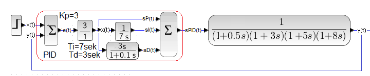
Fig. 28-6
Kp=3 Ti=7 sec Td=3 sec
Fig. 28-7
There is an improvement? Is. Even the overshoot is around 20%. But why did the first shot (Fig. 28-6) miss? I tried clumsily to defend Mr. Ziegler. That this is only the first approximation to the optimal settings. That the parameters Kp, T, To (especially To)were not determined exactly, that … etc.
Chapter 28.3 – Self oscillation method
Chapter 28.3.1 Introduction
In chapter 28.2, we determined the optimal Kp, Ti and Td settings based on the mathematical model describing the object. It doesn’t matter that it was a simplified model – equivalent transmittance Gp(s) of the inertia with delay type in Fig. 28-1. It doesn’t matter that it was based on experiment, not theoretical considerations. It is important that we used the object model. It was the first school of controllers tuning.
The self oscillation method is an example of the second school. No model model is needed here. All you have to do is do “something” to the object and observe its behavior. This “something” can be, for example, a gradual increase in Kp gain in a closed system until it becomes unstable. In other words, it will become a generator.
Chapter 28.3.2 Test No. 1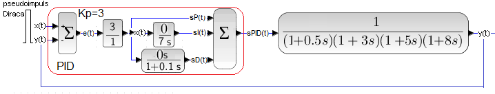
Fig. 28-8
How is it different from Fig. 28-4?
1-Through zeros, the components – integrating and differentiating have been excluded. So the PID controller became the P controller
2-Force x(t) in 3 seconds is now a Dirac pulse (actually a pseudo pulse)
I remind you that unstable systems can “stay still”. Like a sharpened pencil placed upright on a table. It can go on like this until the end of the world, although it is clearly an unstable system. Therefore, to observe instability, we give a Dirac impulse to the input.
Note
The advantage of the method is that it concerns a closed system. “Opening” a closed system in order to study it can be troublesome for an industrial facility.
Fig. 28-9
We hit the object on the nose with a Dirac hammer. It hit and the system returned from the initial state 0 to the final state (equilibrium) 0. So for K=3 the system is stable.
Chapter 28.3.3 Test No. 2
Scheme from Fig. 28-8, only Kp=5
Fig. 28-10
It lingers longer. Conclusion– We have approached instability but the system is still stable.
Chapter 28.3.4 Test No. 3
Scheme from Fig. 28-8, only Kp=6.27
Fig. 28-11
It swings endlessly with a constant amplitude. Conclusion – We are on the verge of stability. What a coincidence that we chose Kp=6.27!
Oscillation period Tosc=16.3 sec.
Let’s remember 2 values from this experiment:
– gain Kp=6.27, which we will call the critical gain Kkr=6.27
– oscillation period Tosc=16.3
Both parameters will be needed to determine the optimal settings Kp, Ti and Td in Chapter. 28.3.7.
We don’t need to increase the Kp gain any more. But let’s do it just out of curiosity.
Chapter 28.3.5 Test No. 5
Scheme from Fig. 28-8, only Kp=6.5
Fig. 28-12
I guess that’s what we expected. The amplitude slowly increases to infinity. If it was a real system and not a linear ideal, the amplitude would increase to +/- saturation.
Chapter 28.3.6 Determination of optimal parameters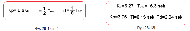
Fig. 28-13
Optimal parameters Kp, Ti and Td are calculated according to very simple patterns–>Fig. 28-13a. They should ensure the shortest control time with an overshoot of no more than 30%. When we substitute Kkr=6.27 and Tosc=16.3 sec from Fig. 28-11 into these formulas, we will obtain optimal settings -> Fig. 28-13b. I suggest checking with a calculator.
Chapter 28.3.7 Step response at optimal settings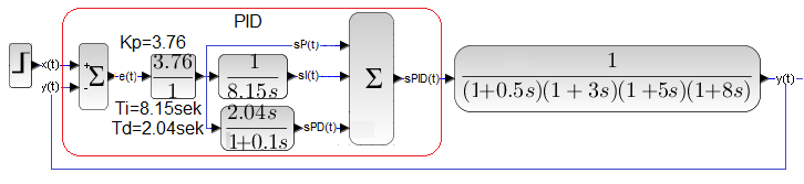
Fig. 28-14
The settings are from Fig. 28-13b, i.e. they are optimal according to the Self Oscillation method
Fig. 28-15
It does not bring you to your knees, but compared to the previous method of step response in Fig.28-5 the response is closer to the optimal one. Of course, this does not mean that the method is better. Maybe it’s different with another facility? I’m not taking a position here.
We can try to correct the parameters manually, so that we get an response not worse than above.