27. PID Control - How does it work?/Jak to dziala?

Automatics

Chapter 27 PID control
Chapter 27.1 Inroduction
We already know that:
– The P control, and even more so the PD control, reacts quickly to the step setpoint x(t), but the steady error e(t) is always non-zero.
– The PI control provides zero control error, but the course is slower than for P control, and even more so for PD control.
The method imposes itself. A differentiating component D should be added to the PI controller. It will turn out that the course will be faster. In addition, the system will be more stable. And what does that mean? That you can, for example, increase the gain Kp of the controller, thanks to which the time chart will be even faster. We will start by examining the structure of the PID controller.

Chapter 27.2 PID controller
This is not yet a controller, because it does not perform its most important function, i.e. the comparison e(t)=x(t)-y(t). For now, the input is only x(t) and we study the dynamics alone.
Chapter 27.2.1 PID unit when x(t) is a unit step

Fig. 27-1
PID unit
Kp=1 Ti=10 sec Td=1 sec
–proportional sP(t)
–integrating sI(t)
–differentiating sD(t)
The input signal is a unit step x(t).
The controller’s sPID(t) signal is the sum of the sP(t) sI(t) and sD(t) components.
The proportional component sP(t) is x(t) because Kp=1.
The integrating component sI(t) increases with such a speed that after time Ti=10 sec. it equals the proportional component sP(t). Here in the 13th second, which you can’t see because the experiment ends in the 10th sec.
The differentiating component sD(t) – In 3 sec, there is a step x(t), i.e. at this time the speed is infinitely great. And this would be sD(t) for the ideal differentiating component D. And it is real! That is, “flattened” by an inertial unit with a time constant Td=0.1 sec. Due to disturbances, the ideal differentiating component D is rarely used.
The components sP(t) and sI(t) are easy to interpret when the input signal x(t) is a step. It is worse with sD(t) because for t=3 sec the signal speed is infinitely high. Therefore, let’s analyze the PID again when x(t) increases linearly.
Chapter 27.2.2 PID unit when x(t) increases linearly x(t)=1t
More strictly x(t)=1t(t-3) because 1t is moved 3sec right
The PID components the same as before.

Fig. 27-2
Kp=1 Ti=10 sec Td=1 sec
The x(t) signal increases linearly–> x(t)=1t(t-3)
The proportional component sP(t) is also equal to x(t) – so it increases linearly
The integral component sI(t) is a parabola function because the integral of x(t) that increases linearly is also some square of time t. It can be seen, though less clearly, in the output signal of the sPID(t) controller.
The real differentiation of sD(t) is clearly visible. The input signal x(t) has been increasing from 3 seconds, but its constant speed was “calculated” with inertia only after about 0.5 seconds. This time is visible on the time chart of the differentiating component sD(t).
Control signal sPID(t) is of course the sum of:
sPID(t)=x(t)+sI(t)+sD(t)
because Kp=1
Previously, i.e. for the x(t) step, it was easy to interpret the integrating Ti and more difficult the differentiating Td.
Now with the “ramp” x(t) it’s the other way around.

Chapter 27.3 PID controller with One-inertial object
Chapter 27.3.1 One-inertial object
The PID controller will be controlled by the same one-inertial object as before, i.e. with a time constant T=10 sec. We will start with the PID controller with the D differentiation action turned off, which is actually the PI controller.
Chapter 27.3.2 PID control Kp=3 Ti=4 sec Td=0 – no differentiation

Fig. 27-3
Kp=3 Ti=4 sek Td=0 sek
that is, it is a PI controller
The process is the same as in Chapter 26 Fig. 26-13 as it applies to the same control systems! So let’s do real PID control by starting with a careful differentiation of Td=0.5 sec.
Chapter 27.3.3 PID control Kp=3 Ti=4 sec. Td=0.5 sec – it’s a real PID!

Rys. 27-4
Kp=3 Ti=4 sek Td=0.5 sek
Where is the positive influence of the derivative? Even longer control time. Let’s increase it to Td=1sec.
Chapter 27.3.4 PID control Kp=3 Ti=4 sec Td=1 sec

Fig. 27-5
Kp=3 Ti=4 sec Td=1 sek
Control time has increased even more. It can be seen that for Kp=3 and the one-inertial unit, the D component does not improve the time chart! Why? At the beginning of the x(t) step, a “spike” of the sPID(t) control signal appears, mainly from the D component. Then the “spike” disappears because it is a real differentiating unit – i.e. with inertia. The entire “pin” is not visible here, because this is the scope of the oscilloscope, but look at, for example, Fig. 27-1. The “pin” almost instantly “raises” y(t). That is, it works well in the direction of speeding up the course. But right after that comes the “inhibiting” component D coming from the increasing y(t). It should prevent overshoots, i.e. y(t) transitions to values greater than 1. For one-inertial units, there are no large y(t) overshoots, which can be seen in the attached picture. What remains, however, is the braking mechanism, which extends the time chart. Slightly but lengthens. Therefore, the PID control for one-inertial objects does not particularly improve the control time. Just PI is enough.
Even better dynamics will be provided by the P control, but unfortunately it will not provide zero error. More about the “accelerating-deceleration” force of the differentiating component D was in Chapter 24 Fig. 24-13.
Chapter 27.3.5 PID control Kp=10 Ti=5 sec. Td=0 sec
As usual, we start with the D component turned off. So we are testing the PI controller. Why Ti=5 sec and not Ti=4 sec as before? Because we found earlier that for the one-inertial unit and the gain Kp=10, the optimal Ti setting for the PI control is Ti=5 sec.

Fig. 27-6
Kp=10 Ti=5 sec Td=0 sec
Best time chart so far. But it’s not because of D , but because of the gain Kp! I feel that Td=0 will be optimal.
Chapter 27.3.6 PID control Kp=10 Ti=5 sec. Td=0.5 sec

Fig. 27-7
Kp=10 Ti=5 sec Td=0.5 sec
Differentiation did not improve the response. Longer control time. Let’s increase the differentiation to Td=1 sec.
Chapter 27.3.7 PID control Kp=10 Ti=5 sek Td=1 sec

Fig. 27-8
Kp=10 Ti=5 sec Td=1 sec
Even worse. So for Kp=10, the best Td setting is Td=0 sec. Similarly to Kp=3.

Chap. 27.4 PID controller with a Two-inertial object
Chap. 27.4.1 Two-inertial Object
A two-inertial object with time constants T1=3 sec and T2=5 sec we have already met. E.g. Chap. 26 Fig.26-20. We will start the with the PID controller with the differentiation action D disabled.
Chapter 27.4.2 PID control Kp=3 Ti=8 sec Td=0 –differentiation disabled
That is PI control

Fig. 27-9
Kp=3 Ti=8 sec Td=0 sec – no differentiation
So let’s do a real PID control, giving a “cautious” differentiation at the beginning – Td=0.5 sec.
Chapter 27.4.3 PID control Kp=3 Ti=8 sec Td=0.5

Fig. 27-10
Kp=3 Ti=8 sec Td=0.5 sec
Finally, PID showed up! Compare the response with the previous one without differentiation. Better. Just as Ronaldo will not show his craftsmanship in the match against a small provincial football club, PID will not impress by controlling a simple one-inertial object. And here is a more difficult to control two-inertial object, and you can see the differentiation effect right away. Let me remind you how the differentiating component D works. At the beginning of the step x(t), the time chart accelerates, because the step x(t) is differentiated. Then it brakes because the differentiating component D additionally (except P and I) reduces the control s(t) signal and thus prevents overshoot. See how effective. Almost no oscillation! Or maybe we can improve the time chart by increasing Td? But first I will show the same time chart with different oscilloscope settings, so that you can see the entire control signal s(t).

Fig. 27-11
I expected it to be “spike”. But that much? Keep this in the back of your mind when you analyze the PID or PD control time charts. What does it mean? The furnace needs e.g. 55 kW to reach a temperature corresponding to y=1. But at the beginning, it gives a power of more than 18 times more, i.e. around 1 MW. Such a small power plant. I don’t think we will give such power to the designed furnace. We are theoreticians for now. We designed system without worrying about limitations. We will return to the topic later in Chapter 31.
Chapter 27.4.4 PID control Kp=3 Ti=8 sec Td=1 sec

Fig. 27-12
Kp=3 Ti=8 sec Td=1 sec
Wonderful, almost no oscillation! Let’s increase Td even more. Maybe we’ll see an even greater miracle.
Chapter 27.4.5 PID control Kp=3 Ti=8 sec. Td=5 sec
We have increased the differentiation from Td=1 sec to Td=5 sec. I wonder what the effect will be?

Fig. 27-13
Kp=3 Ti=8 sec Td=5 sec
Any excess is bad. It is true that, as we expected, the “pin” at the beginning of the x(t) step increased the growth rate of y(t), but then the inhibition due to the strong differentiation of D from y(t) increased. Too strong differentiation of y(t) (“braking”) prevailed over differentiation of x(t) (“accelerating”). It is true that the time chart has become aperiodic (without oscillations), but the control time has increased. We will now start a series of studies of the PID control of a two-inertial object with gain Kp=10. We will start with Td=0, i.e. with the PI control.
Chapter. 27.4.6 PID control Kp=10 Ti=10 sec Td=0 sec.

Fig. 27-14
Kp=10 Ti=10 sec Td=0 sec – differentiation disabled
But it rocks! No customer will issue a VAT invoice for such a control system. Will differentiating D help?
Chapter 27.4.7 PID control Kp=10 Ti=10 sec. Td=0.5 sec
We will start carefully with a gentle differentiation, i.e. from Td=0.5 sec.

Rys. 27-15
Kp=10 Ti=10 sec Td=0.5 sec
It was just a very careful (read-small) differentiation. But how beautifully it calmed down the course. Let’s go this route and increase the differentiation.
Chapter 27.4.8 PID Controller Kp=10 Ti=10 sec Td=1 sec

Fig. 27-16
Kp=10 Ti=10 sec Td=1 sec
Even better! So let’s increase the differentiation to Td=2 sec.
Chapter 27.4.9 PID controller Kp=10 Ti=10 sec Td=2 sec

Fig. 27-17
Kp=10 Ti=10 sek Td=2 sec.
Although we got rid of the overshoot, the zero error occurred only after 25 seconds. It’s like we’re overdoing the differentiation, which is slowing down the time chart. I guess the previous run (Td=1 sec) was the best? Is it? Notice that y(t) very quickly came to a state where e(t)=0.05. Then it decreases very slowly to 0. During this time, mainly integration I works. Or maybe this integration can be accelerated. So let’s take Ti=7 sec. By the way, let’s reduce the differentiation to Td=1.5 sec.
Chapter 27.4.10 PID control Kp=10 Ti=7 sec Td=1.5 sec

Fig. 27-18
Kp=10 Ti=7 sec Td=1.5 sec
Author!!! author!!! Therefore, we will assume the settings of Kp=10 Ti=7 sec Td=1.5 sec of the PID controller as optimal for our two-inertial unit. Compare again this waveform with Fig.27-14 which was carried out by the PI controller. Result as in the Germany-Gibraltar match.

Chap. 27.5 PID controller with a three-inertial object
27.5.1 Introduction
A three-inertial object with time constants T1=0.5 sec T2=3 sec and T3=5 sec we have already met. E.g. Chapter 26 Fig. 26-29. We will start controlling the object with the PID controller with the differentiation D disabled.
Chap. 27.5.2 PID control Kp=3 Ti=10 sec Td=0 sec–differentiation disabled

Fig.27-19
Kp=3 Ti=10 sec Td=0 sec –differentiation disabled
Now let’s do a real PID control, giving a “careful” differentiation at the beginning – Td=0.5 sec.
Chapter 27.5.3 PID control Kp=3 Ti=10 sec Td=0.5 sec

Fig. 27-20
Kp=3 Ti=10 sec Td=0.5 sec
Even such a weak differentiation has a positive effect on the time chart. Let’s check whether it pays off to further increase Td.
Chapter 27.5.4 PID ControllerKp=3 Ti=10 sec Td=1 sec

Fig. 27-21
Kp=3 Ti=10 sec Td=1 sec
Less overshoot and control time improved only slightly. Let’s increase Td.
Chapter 27.5.5 PID Control Kp=3 Ti=10 sec Td=1.5 sec

Fig. 27-22
Kp=3 Ti=10 sec Td=1.5 sec
You can see the “inhibiting” effect of differentiation. A debatable improvement. Plus, there are no overshoots. The downside is that the area under the green e(t) (i.e. the integral of the error) is probably a bit larger. Now let’s move on to Kp=10. To begin with, no differentiation.
Chapter 27.5.6 PID control Kp=10 Ti=10 sec Td=0 sec differentiation D disabled

Fig. 27-23
Kp=10 Ti=10 sec Td=0 sec without differentiation
We expected such oscillations after increasing Kp. In order to “calm down” we will give D differentiation.
Chapter 27.5.7 PID control Kp=10 Ti=10 sec Td=1 sec

Fig. 27-24
Kp=10 Ti=10 sec Td=1 sec
Beautifully. Component D met our expectations. So let’s turn it up Td.
Chapter 27.5.8 PID Control Kp=10 Ti=10 sec Td=2 sec

Fig. 27-25
Kp=10 Ti=10 sec Td=2 sec
Better. The long approach to the steady state e(t)=0 is also irritating. How about increasing the integration speed, e.g. to Ti=7 sec?
Chapter 27.5.9 PID control Kp=10 Ti=7 sec Td=2 sec

Fig. 27-26
Kp=10 Ti=7 sec Td=2 sec
Improvement. And if we compare it with PI control (or PID where Td=0 sec) in Fig. 27-23, it’s a shock! Not to mention the P control. Therefore, we will assume that the optimal settings of the PID controller for the controlled three-inertial object are Kp = 10 Ti = 7 sec Td = 2 sec. They will certainly be better when testing more Kp Ti Td combinations. A lot of studies have been devoted to determining the optimal settings of the PID controller. In chapter 28 we will discuss only the simplest ones.

Chap. 27.6 PID control with disturbances
Chap. 27.6.1 Introduction
The same two- and three-inertial objects will be controlled. We do not study one-inertial ones, because in this case PID is not better than PI. The settings that gave the “prettiest” response will be used. The “prettiest” i.e. relatively fast and with possibly small oscillations. We will call them, with some exaggeration, optimal.
Chapter 27.6.2 Positive disturbance with a two-inertial object z(t)=+0.5 Kp=10 Ti=7sec Td=1.5sec.

Fig.27-27
Optimal controller with respect to x(t), i.e. from Fig. 27-18. The disturbance z(t)=+0.5 will appear in 70 seconds. Up to 70 seconds, the time chart is the same as in Fig. 27-18, of course, taking into account the different time scale on the oscilloscopes. Initially, the disturbance z(t)=+0.5 caused an increase in the y(t) signal, but then the control signal sPID(t) “forced” y(t) to return to the previous value, i.e. to y(t)=1. This corresponds to the appropriate reduction of the error e(t) to 0. It is clearly visible how the steady-state PID controller reacted with cooling sPID(t)=-0.5 to the additional heating z(t)=+0.5. The D component improves the dynamics of the course.
Note
In response to the disturbance z(t)=+0.5, the control signal sPID(t) coincides in steady state with the disturbance z(t)=+0.5. This also applies to the following examples where z(t)=+0.5.
Chapter 27.6.3 Negative disturbance with a two-inertial object z(t)=-0.5 Kp=10 Ti=7sec Td=1.5sec.

Fig. 27-28
The disturbance z(t)=-0.5 will appear in 70 seconds.
Initially, the disturbance z(t)=-0.5 caused a decrease in the y(t) signal, but then the control signal sPID(t) “forced” y(t) to return to the previous value, i.e. to y(t)=1. This corresponds to the appropriate reduction of the error e(t) to 0. The negative interference – “cooling”, the sPID(t) control responded by increasing the power – “heating“.
Chapter 27.6.4 Positive disturbance with a three-inertial object z(t)=+0.5 Kp=10 Ti=7sec Td=2sec.

Fig. 27-29
The disturbance z(t)=+0.5 will appear in 70 seconds.
The object is more difficult to control, and although PID makes more contortions than for the two-inertial one, the effect is slightly worse. I leave the analysis of the next experiment with negative interference z(t)=-0.5 to the reader
Chapter 27.6.5 Negative disturbance with a three-inertial object z(t)=-0.5 Kp=10 Ti=7sec Td=2sec.

Fig. 27-30
The disturbance z(t)=-0.5 will appear in 70 seconds.

Chapter 27.7 Comparison of P, PD, PI and PID controllers
27.7.1 Introduction
We will compare the P, PD, PI and PID controls while giving the step x(t) to 4 control systems controlling the same object:
– two-inertial
– three-inertial
The optimal settings for setpoint x(t) of the controllers were selected by us earlier.
Chapter 27.7.2 Control systems with a two-inertial object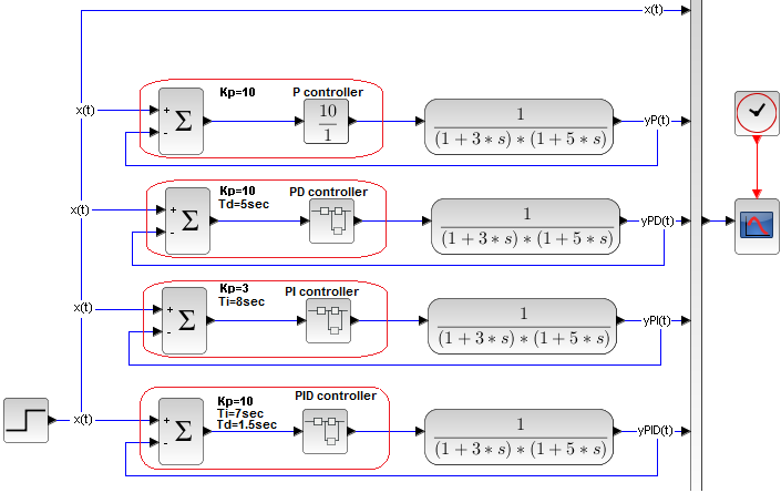

Fig. 27-31
Previously, you examined these objects with optimal settings in the chapters:
– 26 P control
– 27 PD control
– 29 PI control
– 30 PID control
Here we have their poorer versions with a common input signal x(t) and a single output yP(t), yPD(t), yPI(t) and yPID(t) from each controlled object.

Fig. 27-32
The black yP(t) of the P control is the worst. It has the most oscillations, lasts a long time and does not provide zero error.
The green yPD(t) of the PD control has the best dynamics – an almost rectangular response. It also does not provide zero error.
The blue yPI(t) of the PI control already provides zero error, but long control time and oscillations
The red yPID(t) has the most advantages. Zero error, short control time and low oscillation.
Now compare the effects of work of the cool PID controller and its poor relative P.
Chapter 27.7.3 Control systems with a three-inertial object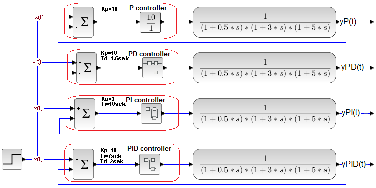

Fig. 27-33

Fig. 27-34
The time charts are worse than before, because the object itself is more difficult to control. The general conclusions remain the same.

Chapter 27.8 Conclusions of the PID Control
PID is the king of all controllers. Even for some, the terms PID and controller mean the same thing. Just like electrolux and vacuum cleaner.
The concept of PID did not come from sophisticated mathematical considerations, but from simple observations. For example, how the helmsman tries to keep the ship on course despite disturbances such as waves, wind. Also, the change of course is nothing more than the response of the control system to a unit step.
In everyday life, a person uses a PID algorithm in which the component:
–P is an immediate reaction to an event typical of young people
–I is a reaction that takes into account life experience with similar cases in the past. Don’t be nervous, react gradually. If something bothers you (error e(t)), gently act in the right direction and wait for the effects. Typical of the elderly people.
–D is the ability to predict the future. The response is proportional to the tendency of the phenomenon. The setpoint value x(t) increases, so my reaction results not only from the set setpoint value x(t) itself, but also from its speed. On the other hand, when x(t) is established, in order to prevent overshoots, I start braking even when y(t) has not yet reached the setpoint x(t). Because y(t) is growing too fast!
PID type reactions apply not only to technology.
In economics, a broker makes a decision to buy/sell shares of a given company at a price that will result from:
– current stock price–>(P)
– knowledge about the history behavior of the shares, more broadly the company–>(I)
– trend of price increase/decrease–>(D)
For a complete analogy, buying shares is a positive control signal and selling a negative one.
There are brokers to whom you would entrust your money (well-tuned PID controllers) and bad ones