25. I Control - How does it work?/Jak to dziala?

Automatics

Chapter 25 I Control
Chapter 25.1 Introduction
You have already met the simplest type P controller consisting only of a comparator element and an amplifier Kp. It roughly ensured approaching the setpoint x(t) and suppressing disturbances z(t). Then came the PD controller which did the same thing, only much faster and with smaller oscillations. Still, however, the steady-state closed-loop gain Kz and the error gain Ku was as follows:

Fig. 25-1
The formulas show that Kz is always slightly smaller than 1. The closer to 1, the larger K. Similarly, Ke is always slightly larger than 0. The closer to 0, the larger K. Let me remind you that K is the steady gain of the entire open control system. That is, taking into account the Kp of the controller and the Ko of the object. It so happens that it is mostly Ko=1, then K=Kp. It is convenient when selecting the controller settings–> chapter 31.
And now the most important!
For type I control, the formulas for Kz and Ke are as follows:

Fig. 25-2
Cheaper, sorry, it couldn’t be easier! And what does that mean? If we enter x(t) in the form of a unit step, then after some time it will be y(t)=x(t). So error e(t)=0! This is the main goal of every automatics engineer. The control time may be long, and there may also be fading oscillations. But when certain additional conditions are met (Hurwitz!, Nyquist!…) this will always happen. And when they are not fulfilled? Then the system is unstable.
Note
The formulas in Fig. 25-2 are actually a special case of Fig. 25-1. Because what is the gain K of the object with the integral unit in steady state. y(t)=infinity when t=infinity! So K=infinity! Substitute this value into Fig. 25-1 and you will get Fig. 25-2.
The I controller consists of a comparison element and an I integrating element with adjustable integration time Ti. It is rarely used as a standalone controller. The integral unit I, however, is present in the PI or PID controllers and its purpose is to bring the error e(t) to zero.
You’ve met I unit him earlier in chapter 4, but I suggest a quick replay!

Chapter 25.2 Integral unit
Chapter 25.2.1 Introduction
We will examine 3 units I with different integration rates
-Slow
-So so
-Fast
They are not yet I controllers, because they do not have a comparator that calculates the error e(t)=x(t)-y(t)
Chapter 25.2.2 Slow I unit Ti=2sec

Fig. 25-3
Ti=2sec
The integral unit with the integration time Ti=2sec. The signal increases at a constant rate. Ti=2sec is the time after which y(t) equals the step x(t).
Chapter 25.2.3 “So so” I unit Ti=1 sec

Fig. 25-4
Ti=1 sek
After time Ti=1 sec, y(t) equaled the step x(t). That is 2 times faster than before.
Chapter 25.2.4 Fast I unit Ti=0.5sec

Fig. 25-5
Ti=0.5 sec.
After the time Ti=0.5 sec y(t) equaled the step x(t). Again 2 times faster than before.

Chapter 25.3 Servo controller that reduces e(t) error to 0 as an example of I control
Chap. 25.3.1 Introduction
This is a good example that type I control reduces the e(t) error to 0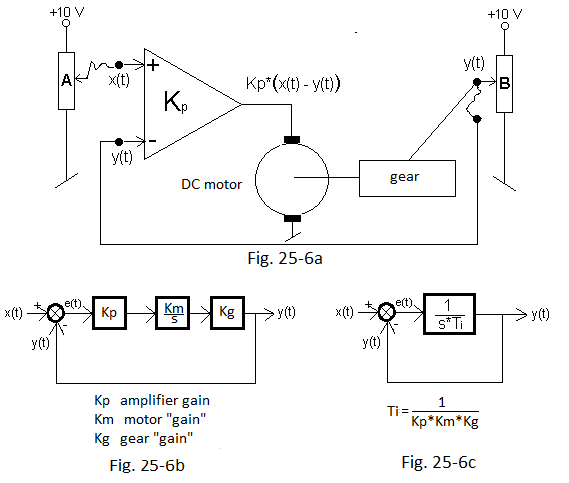

Fig. 25-6
The input is the voltage x(t) across potentiometer A Fig. 25-6a. The DC motor is controlled by the voltage difference e(t)=x(t)-y(t). The motor shaft is mechanically coupled through a gear with the slider of the potentiometer B. The motor is ideal, i.e. when there is a voltage on it even as small as +1 µV, the slider will slowly move up, i.e. the voltage y(t) will slowly increase. And when +2 µV is +2 times faster. Similarly -1 µV the slider will go down. This is the classical integrating unit, i.e. the I unit.
Slider B will only stop in one situation. When x(t)=y(t), i.e. when the voltage on the motor is zero.
At first, both sliders are down. So x(t)=y(t)=0V and the voltage on the motor is also zero, because Kp*[x(t)-y(t)]= Kp*(0-0)V=0V and the motor stops. Suddenly you will set potentiometer A +5V. As if you gave a unit step x(t)=+5V Then the motor will go up with a high initial speed. The speed will decrease, because at the input – of the amplifier there will be a voltage “subtracting” from the slider. b
In this way, slider B will reach +5V after a theoretically infinite time. The voltage on the motor will be zero.
And what if the gear motor had inertia and the slider would exceed +5V. For example, it would be +5.1V. Then a negative voltage will appear and the slider B will move back towards +5V, until after some time it will be back to +5V.
That’s how it is in an ideal world. In real life, there are some hysteresis, dead zones and other clutter, so that the slider would be set to, for example, +4.999V. Then the very small voltage on the motor would not be able to move it.
So you see that under ideal assumptions the error will be zero, which is typical for type I control.
Fig. 25-6b is a block version of the diagram in Fig. 25-6a. Here the Kp of the amplifier is obvious. The motor’s Km is greater the higher the speed of the motor at a given voltage. The Kg parameter of the gear is like a derailleur in a bicycle.
In total, it is an integral unit with some integration time Ti covered by a negative feedback loop–>Fig. 25-6c.
Chapter 25.3.2 Slow servo model
The servo control boils down to the very simple Fig. 25-6c.

Fig. 25-7
The input x(t) is the voltage x(t) across potentiometer A Fig. 25-6a. The DC motor is controlled by the voltage difference e(t)=x(t)-y(t). The motor shaft is mechanically coupled through a gear with the slider of the potentiometer B. The motor is ideal, i.e. when there is a voltage on it even as small as +1 µV, the slider will slowly move up, i.e. the voltage y(t) will slowly increase . And when +2 µV is +2 times faster. similarly -1 µV the slider will go down. This is the classical integrating term, i.e. the I unit.
Slider B will only stop in one situation. When x(t)=y(t), i.e. when the voltage on the motor is zero.
At first, both sliders are down. So x(t)=y(t)=0V and the voltage on the motor is also zero, because Kp*[x(t)-y(t)]= Kp*(0-0)V=0V and the motor stops. Suddenly you will set potentiometer A +5V. As if you gave a unit step x(t)=+5V Then the motor will go up with a high initial speed. In a moment the speed will decrease, because at the input – of the amplifier there will be a voltage “subtracting” from the slider. b
In this way, slider B will reach +5V after a theoretically infinite time. The voltage on the motor will be zero.
And what if the gear motor had inertia and the slider would exceed +5V. For example, it would be +5.1V. Then a negative voltage will appear and the slider B will move back towards +5V, until after some time it will be back to +5V.
That’s how it is in an ideal world. In real life, there are some hysteresis, dead zones and other clutter, so that the slider would be set to, for example, +4.999V. Then the very small voltage on the motor would not be able to move it.
So you see that under ideal assumptions the error will be zero, which is typical for type I control.
Fig. 25-6b is a block version of the diagram in Fig. 25-6a. Here the Kp of the amplifier is obvious. The motor’s Km is greater the higher the speed of the motor at a given voltage. The Kg parameter of the gear is like a derailleur in a bicycle.
In total, it is an integralunit with some integration time Ti covered by a negative feedback loop–>Fig. 25-6c.
Chapter 25.3.3 Slow servo control
The servo control boils down to the very simple diagram in Fig. 25-6c.

Fig. 25-8
Servo model when Ti=1 sec
The system reacted 4 times faster. It reached the steady state y(t)=7.5 V after about 7.5 seconds.
Chapter 25.3.4 Conclusions from the servo test
Integration I appeared in the control system, because the DC motor is an integrating unit. This brought the error e(t) to zero. This is the most important advantage of integration. In previous chapters, the proportional component P was unable to reduce the error to 0. Here, the I component did it. Because no matter how small the error is, even a very small voltage will always spin the motor so that y(t)=x(t). Of course, theoretically. In practice, however, the deadband and hysteresis of the motor will cause some error.

Chapter 25.4 I control with an one-inertial object
Chapter 25.4.1 Introduction
We will examine a system in which the I controller controls an inertial object with a time constant T=10 sec. We will start with the most conservative setting Ti=36 sec, then Ti=16 sec and finish with Ti=8 sec. Patience will be required as the experience time is 2 minutes. We will start, as usual, with the study of the inertial object itself.

Fig. 25-9
An inertial object with a time constant T=10 sec.
Chapter 25.4.2 I control Ti=36 sec

Fig. 25-10
The only setting of the controller is Ti=36 sec. We start with such a slow integration, because we are afraid of oscillations and even instability. I guess the fears were exaggerated. The system very slowly came without oscillations (in other words – aperiodically) to the state of equilibrium, where x(t)=y(t). So error e(t)=0. In fact, after 120 seconds, the state y(t)=1 is not yet there. It will happen later. But I guess you believe it will. As long as the error e(t) is different from 0 (here more than 0), the I controller will push the signal to the state where y(t)=x(t)=1. In theory, it’s infinitely long, in practice after about 130 seconds.
Chapter 25.4.3 Control I when Ti=16 sec
The previous run was slow. Faster integration Ti=16 should improve the situation.

Fig. 25-11
I control Ti=16 sec
Great joy at first. As s(t) grows faster, y(t) does the same. Unfortunately, there was an oscillation. Nevertheless, after about 120 seconds, the output signal y(t) reached the state of equilibrium, in which, as the steady-state error is zero. Is the response much better than the previous one? Suppose it does despite the oscillation.
Chapter 25.4.4 I control Ti=8 sec
Let’s shorten thecontrol time even more by giving Ti=8. Maybe it will be better?

Fig. 25-12
I control Ti=8 sec
Slightly shorter control time but larger oscillations. We will therefore assume that the setting Ti=16 sec is optimal for the inertial unit with the time constant T=10 sec.

Chapter 25.5 I control with an Two-inertial object
Chapter 25.5.1 Introduction
The I control controls the two-inertial object. We will start with the study of the object itself. Already the two-inertial object turned out to be difficult to control, long control time and oscillations. It will probably be even worse here.

Fig. 25-13
Two-inertial object with time constants T1=3 sec and T2=5 sec
You can see the inflection point characteristic of multi-inertial objects. It is difficult to read the parameters T1=3sec and T2=5sec from the time chart.
There are ways to do it, but let’s just give it a rest.
Chapter 25.5.2 Control I when Ti=25 sec

Fig. 25-14
I control Ti=25sec
Surprise. The time chart is’nt better or worse than “easier” I control for the one-inertial unit from Fig. 25-11! I was prepared for the worse answer y(t). Can someone explain it?
Chapter 25.5.3 Control I when Ti=15 sec

Fig. 25-15
If we don’t care about oscillations, it’s better. Shorter adjustment time.
Chapter 25.5.4 Control I when Ti=6 sec

Rys. 25-16
I control Ti=6 sek
However, we overdid it. Not only is it a long control time, but dangling is unacceptable. We will therefore assume that the setting Ti=15 sec is optimal for the two-inertial unit with time constants T1=3 sec and T2=5 sec.

Chapter 25.6 I control with an three-inertial object
Chapter 25.6.1 Introduction
First, the object itself.

Fig. 25-17
A three-inertial object with time constants T1=0.5 sec, T2=3 sec and T3=5 sec.
The response is similar for the two-inertial one in Fig. 25-13, although we know very well that the three-inertial one is more difficult to control.
Chapter 25.6.2 I control Ti=30 sec
We will start with careful control, i.e. slow integration Ti=30 sec.

Fig. 25-18
Control I Ti=30 sec
This shows careful control. The control signal s(t) is slightly larger than y(t).
Just like a teacher who is undemanding to the student. Therefore, the response is slow and without oscillation.
Chapter 25.6.3 I control Ti=10 sec

Fig. 25-19
I Control Ti=10 sec
Control time shorter although oscillations appeared.
Chapter 25.6.4 I control Ti=5 sec

Fig. 25-20
I control I Ti=5 sek
Terrible oscillations. We will therefore assume that the setting Ti=10 sec is optimal for this three-inertial unit
Chapter 25.6.5 When we overdo the integration i.e. Ti=1.5sec
So with the speed of integration, e.g. Ti = 1.5 sec

Fig. 25-21
I control Ti=1.5 sek
You can’t see it, but there is a different oscilloscope scale. Can you guess why?
Beautiful instability. The oscillation amplitude increases to +/-infinity.

Chapter 25.7 I control with disturbances
Chapter 25.7.1 Introduction
The same 3 objects will be controlled. Their inputs will be affected by large disturbances z(t)=+0.5 or z(t)=-0.5. The resulting error e(t) will “annoy” the integrating component I so much that it will always bring it to e(t)=0. You just need to be patient, because due to the slow time charts typical of type I control, the experiments will last up to 4 minutes!
Chapter 25.7.2 Positive disturbance with a one-inertial object z(t)=+0.5, Ti=16sec

Fig. 25-22
The disturbance z(t)=+0.5 will appear in 130 seconds.
Up to 130 seconds, i.e. until the appearance of a disturbance, the waveform is the same as in Fig. 25-11, taking into account, of course, a different time scale on oscilloscopes. Initially, the disturbance z(t)=+0.5 caused an increase in the y(t) signal, but then the I component “forced” y(t) to return to its previous value, i.e. to y(t)=1. This corresponds to the appropriate reduction of the error e(t) to 0. The positive disturbance-“heating”, the control s(t) responded with a reduction in power.
Chapter 25.7.3 Negative disturbance with a one-inertial object z(t)=-0.5, Ti=16sec

Fig. 25-23
The disturbance z(t)=-0.5 will occur at 130 seconds.
On the negative disturbance – “cooling”, the control s(t) reacted by increasing the power. The error e(t) was reduced to 0.
Chapter 25.7.4 Positive disturbance with a two-inertial object z(t)=+0.5, Ti=15sec.

Fig. 25-24
The disturbance z(t)=+0.5 will occur at 130 seconds.
For a positive disturbance z(t)=+0.5 – “heating”, control s(t) reacted with power reduction.
Chapter 25.7.5 Negative disturbance with a two-inertial object z(t)=-0.5, Ti=15sec

Fig. 25-25
The disturbance z(t)=-0.5 will occur at 130 seconds.
On the negative disturbance – “cooling”, the control s(t) reacted by increasing the power.
Chapter 25.7.6 Positive disturbance with a three-inertial object z(t)=+0.5, Ti=10sec

Fig. 25-26
The disturbance z(t)=+0.5 will occur at 130 seconds.
On a positive positive disturbance z(t) – “heating”, the control s(t) reacted with a reduction in power.
Chapter 25.7.7 Negative disturbance with a three-inertial object z(t)=-0.5, Ti=10sec

Fig. 25-27
The disturbance z(t)=-0.5 will occur at 130 seconds.
On the negative disturbance z(t) – “cooling”, the control s(t) reacted by increasing the power.

Chap. 25.8 Comparing Type I, P and PD Regulations.
Chap. 25.8.1 Introduction
PD, P and I type regulators will control the two-inertial object. Their inputs will receive unit steps x(t) in 3 seconds, and positive disturbance z(t)=+0.5 or negative disturbance z(t)=-0.5 in 120 seconds.
We will compare the output signals y1(t), y2(t) and y3(t), especially their steady states and control times. We will only observe a unit step x(t), a disturbance z(t) and 3 output signals y1(t), y2(t) and y3(t). Missed e(t) and s(t) signals have already been observed in previous experiments.
Chapter 25.8.2 Positive disturbance z(t)=+0.5.
PD, P and I type regulators will control the two-inertial object. Their inputs will receive unit steps x(t) in 3 seconds, and positive disturbance z(t)=+0.5 or negative disturbance z(t)=-0.5 in 120 seconds.
We will compare the output signals y1(t), y2(t) and y3(t), especially their steady states and control times. We will only observe a unit steps x(t), a disurbance z(t) and 3 output signals y1(t), y2(t) and y3(t). Missed e(t) and s(t) signals have already been observed in previous experiments.
Chap. 25.8.3 Positive disturbance z(t)=+0.5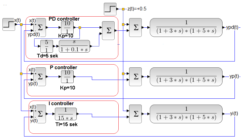

Fig. 25-28
The controller settings Kp=10 of the PD and P controllers according to the formula for Ke in Fig.25-1 will provide a steady state e(t)=9%. In addition, setting Td=5 sec of the PDcontroller will give us the shortest possible control time with a small overshoot.
The I controller ensures zero steady state error e(t) regardless of the Ti setting.

Fig. 25-29
PD–green control is the fastest, although it gives a non-zero steady error e(t).
P–blue control is slower and with overshoots and also gives the same non-zero steady error e(t).
I–red control is the slowest, but provides zero steady error e(t). And this is the basic advantage of type I, i.e. integral, control.
Chap. 25.8.4 Negative disturbance z(t)=-0.5
The scheme is the same as in Fig. 25-28, only negative disturbance, i.e. z(t)=-0.5.

Fig. 25-30
I leave the analysis to the reader.

Chapter 25.9 Conclusions
Why is type I control so slow? Look at the control signals s(t) in earlier experiments. For P and even more so for PD they are large at the beginning of x(t) and z(t). This is what determines the quick control time. In addition, in the case of PD, the derivative component gives a braking effect that prevents oscillations. Control I does not have this initial kick s(t).
What should be done so that the system reaches a steady state relatively quickly, but with a zero steady-state error? The method imposes itself.
Combination of the P controller with the I controller resulting in the PI controller–>chapter 26.
Or even better – a combination of PD with an I controller giving a PID controller–>chapter 27.