Automatics

Chapter 21 On-Off Control
Chapter 21.1 Introduction
Before we get to know the PID control, in this chapter we will discuss the operation of the easiest control. This is On-Off Control. We will start with the relay and the related concept of the so-called hysteresis.

Chapter 21.2 Relay as a ON-OFF element without hysteresis

Fig. 21-1
The relay algorithm is trivial
x(t>0–>On
x(t)<0–>Off
Depending on what is connected to the relay contacts, ON and OFF means different things. Here, for example
ON–>y(t)=1–>U=∼230V heating
OFF–>y(t)=0–>U=0 cooling*
*cooling may also be more intense. e.g. turning on the fridge compressor
The animation is so clear that it needs no further comments.

Chapter 21.4 Man as a ON-OFF controller
Let’s draw a control diagram with you as the controller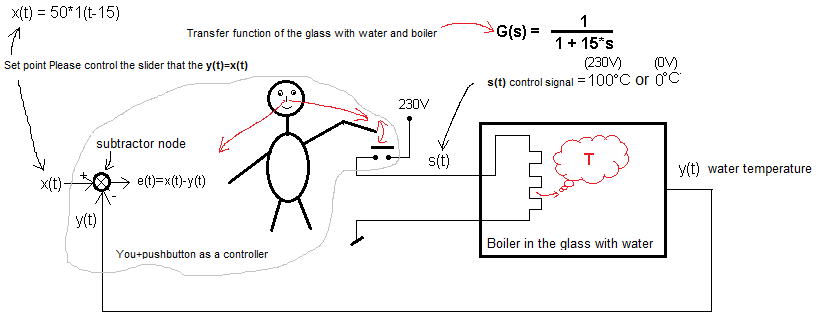

Fig. 21-3
Treat a glass of water like an object. You, as the regulator, try to maintain the water temperature y(t)=+50°C by switching the heater on and off. Since you are an outstanding electronics engineer, you came up with a brilliant idea to replace the “insertion and removal” of the heater plug with a control button with normally open contacts -> those that are open without voltage.
Note:
1(t-15) this is the so-called  step unit which:
1(t-15)=0 dla t<15sek
1(1-15)=1 dla t>15sek
The control algorithm is trivial.
– x(t)>y(t) –> turn on the heater
– x(t)<y(t) –> turn off the heater
Since e(t)=x(t)-y(t) we will replace the above-mentioned algorithm with the following:
– e(t)>0 –> turn on the heater
– e(t)<0 –> turn off the heater
The control signal turn on the heater corresponds to the signal s(t)=230V. The power of the heater is selected so that the steady state water temperature reaches y(t)=+100°C. If the power of this heater was a little lower, we would get a lower temperature. e.g. y(t)=+99°C. Therefore, the command turn on the heater can be replaced with a control signal s(t)=+100°C.
Similarly, turn off the heater can be replaced with s(t)=0°C. We assume that the temperature of the air around the glass is 0°C. So when the heater is turned off, the water temperature will tend to 0°C.
The control algorithm will now be as follows:
e(t) = x(t)-y(t)
– e(t)>0 –>s(t)=+100°C (turn on the heater)
– e(t)<0 –> s(t)=0°C (turn off the heater)
The e(t) value is called the control error and is “calculated” in your head, which serves as the so-called subtractor node. The process is fast and you are not able to calculate that e(t)=50°C-37.5°C=12.5°C at a given moment. It is because of your imperfections. You can only approximately determine the sign of the error e(t). Then, with some delay, because you don’t have the swordsman’s reflexes, you make a decision as to whether to turn on/off the voltage on the heater.
You have learned the most important concepts of automatics
– Setpoint x(t). The value that the controller tries to maintain at the object output. The x(t) here is +50°C
– Process variable or output signal y(t). The value on the output of the object that the controller managed to provide
– Control error, that is e(t)=x(t)-y(t) This is a measure of the “imperfection” of the controller. For an ideal, it should be e(t)=0. It is calculated in the so-called subtractor node.
– The control signal s(t) is fed directly to the object input.
An ideal controller provides the same value y(t) at the output as the setpoint x(t). So it ensures e(t)=0.
Like any ideal, the ideal controller does not exist. Maybe that’s good? If you were in a train whose speed changes by leaps and bounds, the acceleration would be infinitely great for a while. It would end badly for you.

Chapter 21.5 On-Off control system
The manual control system in Fig. 21-3 can be easily replaced with an automatic control system. The role of the subtraction node is performed by the operational amplifier WO. It performs the operation e(t)=x(t)-y(t).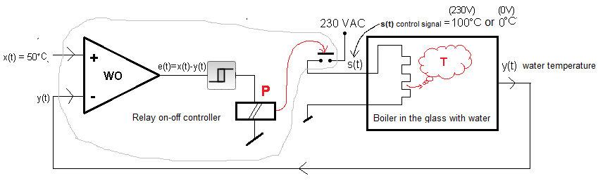

Fig. 21-4
On-Off control system with a relay
It does the same as you in Fig. 21-3, only more precisely and more clearly.
We will slightly modify the control algorithm. What for? It’ll clear up in a moment.
– e(t)>+5°C –>s(t)=+100°C (turn on the heater)
– e(t)<-5°C –> s(t)=0°C (turn off the heater)
Switching on occurs at a different value than switching off. This is what the hysteresis you learned earlier is for.

Chapter 21.6 On-Off Control Test
Chapter 21.6.1 Introduction
We will investigate the influence of:
– Set point x(t)
– Hysteresis
– Heating power
– Cooling power
Chapter 21.6.2 Setpoint step x(t), hysteresis +5/-5

Fig. 21-5
The diagram is a representation of the diagram in Fig. 21-4. So where did the relay with the contact and the voltage of 230V go? I just assumed that everything fits in the hysteresis unit. I set the hysteresis -5°C … +5°C and control signals s(t)=0°C and s(t)=100°C as equivalents of on when e>+5º and off. when e<-5º. In this way, the output signal y(t) will increase to +100ºC (before it starts to decrease) and decrease to 0ºC (before it starts to increase) around the step setpoint signal x(t).
The first activation is obvious because e(t)>+5°C. The temperature y(t) starts to increase and the error e(t) will first jump to +50°C and then decrease. Then there will be a series of switching ON when e<-5º and switching OFF when e>+5º. in this way, the output-temperature y(t) will oscillate in the range -45°C…+55°C, i.e. around +50°C.

Chapter 21.6.3 “Steps” set value x(t), hysteresis +5/-5
And what will happen if the set value x(t) changes during the experiment?

Fig. 21-6
We study the same system, only the time chart of the set point x(t) is different.
You also have to be patient, the experiment lasts 3 minutes instead of 1.
The waveforms show that when:
x(t)=0°C is 0% of maximum power (no heating)
x(t)=+25°C is 25% of the average maximum power (in steady state 25% of the heating time, 75% of the cooling time)
x(t)=+50°C is 50% of the average maximum power (in steady state 50% of the heating time, 50% of the cooling time)
x(t)=+75°C is 75% of the average maximum power (in steady state 75% of the heating time, 25% of the cooling time)
x(t)=+100°C is 100% of the average maximum power (in steady state 100% of the time heating and no cooling). We haven’t done the last experiment (x(t)=+100°C) , but it’s easy to imagine.
We didn’t do a thorough thermal analysis of a glass of water with a glass. Specific heat of water, glass and other “calories”. The only thing we took care of is the minimum power of the heater, which will ensure that the water is heated to 100°C. And yet the system delivers as much energy to the glass as it needs. So automatics allows you to control the object, not fully known out by us.
The controller “forces” the red output signal y(t) to follow the black setpoint signal x(t). The measure of the imperfection of the controller is the green error signal e(t). The effect of this “forcing” is manifested in the fact that the green error e(t) always tends to a state in which it will be inside the hysteresis bar -5°C … +5°C.
I once mentioned that an ideal controller reproduces exactly the set value x(t) at the output y(t). Then the green error e(t) would be zero all the time. I did not expect such an ideal, but the y(t) waveform does not throw Although the output signal y(t) at least tries to reproduce the input signal x(t).
The main “allegations” against the “accused” controller are:
-temperature oscillations at the output (“teeths”)
– too slow approach to the set value x(t). Let’s try to make it better. First the “teeths”.
Chapter 21.6.4 Setpoint step x(t), hysteresis +1/-1

Fig. 21-7
The diagram differs from Fig. 21-5 as follows:
– 5 times less hysteresis – barely visible as yellow +1 and -1 lines
– Single input impulse instead of unit step.
Reducing the hysteresis reduces the oscillations (“teeth”) at the output. You can barely see the bar with the yellow hysteresis lines +1…-1 now. Unfortunately, nothing in life is free. When the regulator controls e.g. contactors, such “clicking” every second will quickly spoil them.
What about semiconductor switching (triacs, transistors, thyristors…)? You can do this when controlling the heater. But when there is, for example, an electric motor on the way like in a refrigerator? Then you have to be careful. In addition, we can reduce the hysteresis even to zero (ideal relay), and the oscillations will remain. And this is because the dynamic unit of the “furnace” type, in addition to the inertia T, also have a delay To.
Also note the “slower” fall of y(t) after 30 seconds than its “faster” increase after 5 seconds. The matter is simple. After 5 seconds, the initial value is y(t)=0°C and the goal it is striving for is y(t)=+100°C. After 30 seconds, the initial value is y(t)=+50°C and the goal it strives for is y(t)=0°C. The goal is now 2 times less ambitious and therefore y(t) is 2 times slower.
We managed to reduce the “teeth”. Now it’s time to get to the set temperature +50°C faster.
Chapter 21.6.5 Square pulse setpoint, hysteresis +5/-5, increased heating power

Fig. 21-8
For didactic reasons, we returned to the previous wider hysteresis. It’s just easier to see what’s going on then. The solution to the problem is self-evident. The heater power has been increased 2.5 times – the “positive” output of the hysteresis element has been increased to +250°C. So as if the water was now to reach +250°C during heating and not +100°C. Let’s not discuss the fact that with ordinary pressure, the max. temperature for water is +100 ° C, etc … We know what’s going on.
For obvious reasons, the temperature now reaches +50°C much faster. Despite the use of a more powerful heater, we will pay about the same for energy. Although the “heating” pulses now have a larger amplitude, they last shorter than the previous one. The energy or field of the control signal s(t) will remain roughly the same.
The temperature quickly reaches the set value +50°C. It was forced by “stronger” heating. However, returning to 0°C takes as long as before. Now and then cooling is done by power supply off.
How about additional cooling, instead of a simple power off?
Chapter 21.6.6 Square pulse setpoint, hysteresis +5/-5, increased heating and cooling power 
Let’s go all the way, let’s cool -250 ° C!. So instead of just turning off the heater, I pass, for example, some liquefied gas at -250°C through the coil!
Let’s assume one more. In the glass we have not water, but some kind of liquid that can be cooled to -250°C and heated to +250°C.
Why this assumption? So as not to enter into digressions about what will happen below 0°C when the water freezes and above +100°C when the water boils.
The diagram is similar to Fig. 21-8, only the hysteresis term for e<-5°C now gives -250°C (instead of 0°C). You can see it on Fig.21-10.

Fig. 21-9
I’m getting scared, we’ve created Frankenstein. The most important thing is that the goal has been achieved. The temperature quickly reaches +50°C and 0°C. But at what cost. For x(t) = 0°C, there are constant oscillations, with a filling of 50%. It eats up energy all the time!
Sometimes control with active heating and cooling is used. For example, for cold rooms used to test aircraft parts, which change from a temperature of e.g. +30°C to -70°C in a few minutes. Here I remembered my first job at the Institute of Aviation.
The blue control signal muddies the picture a bit. Let’s show the same thing, but only for 2 signals x(t) and y(t).
Note:
The zero temperature y(t)=0ºC is ensured by alternating pulses of +250ºC and -250ºC. This is a disaster in terms of energy efficiency, but this control provides the best process dynamics.

Fig. 21-10
Equivalent to Fig. 21-9 only for the two most important signals. You can see how the temperature at the output y(t) “listens to” or rather tries to “listen to” the set point x(t). The control signal s(t), which muddied the image in Fig. 21-9, is absent, but you can imagine it by observing the “teeth” y(t):
s(t)=+250°C when y(t) increases
s(t)=-250°C when  y(t) decreases
And when the setpoint changes several times?
Chapter 21.6.7 “Stairs setpoint” hysteresis +5/-5, increased heating and cooling power
It will be a simplified scheme, with only 2 signals x(t) and y(t). Now the single pulse x(t) in Fig. 21-10 has been replaced with “steps”.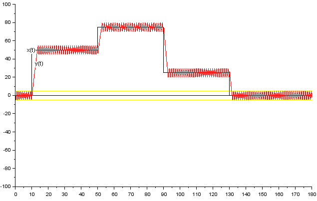

Fig. 21-11
It is beautiful to see how y(t) follows x(t). Maybe a little annoying is the phenomenon of “teeth”. This is due to the big hysteresis -5…+5, which was set only for didactic reasons. If we gave -1…+1, the oscillations would be smaller and of higher frequency. You would see a red line with a thickness of -1…+1.
The control signal  s(t) is also a bit scary. The liquid in the glass (not water!) is heated up to +250°C and cooled down to -250°C every second. But the goal has been achieved! The temperature y(t) follows more x(t) than in Fig. 21-6, where the control was “softer” +100°C/0°C. This corresponds to the general principle of automatics. Stronger negative feedback results in more accurate and faster control. Of course, as long as you don’t overdo it leading to instability
The controller tries to keep the water temperature equal to the set point  x(t).
It does it in a primitive way:
too cold –> heat
too hot –> cool
but somehow he manages.
What if there was mercury instead of water? Mercury has a higher specific heat , or in “human voice” – it takes longer to heat up and cool down. It would take longer to reach the set point, but it would also stabilize. Why? Because the regulator is not interested in what is heating, but makes a control decision based on the current temperature.
What if you add some cold liquid to the glass? The controller won’t even know what caused the temperature drop, it will only decide to add additional heating. And again, it will try to keep the water temperature at a value equal to the set value.
I forgot to add that everything will work out, provided that we ensure the proper power of the heater. After all, it is not possible to use a small “glass” heater powered by a battery to keep the water temperature in the bathtub at, for example, +50°C, even if the regulator told you to heat it all the time.
This brings us to the basic task of automation. It is disturbances suppression.

Chap. 21.7 Disturbance in an open system
21.7.1 Introduction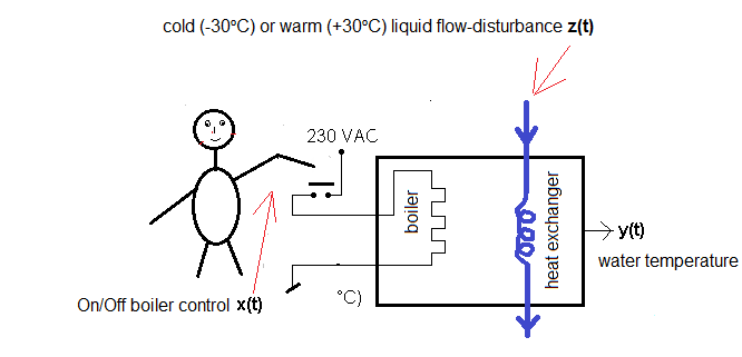

Fig. 21-12
A glass of water with 2 input signals
-x(t) control signal from the boiler
-z(t) disturbance signal from the heat exchanger
and with 1 output signal
-y(t) water temperature
The issue of disturbances applies to any type of control, not only on-off type. Remember this when we move on to the continuous PID control
As you will see, an open system is completely vulnerable to disturbances. Imagine that your refrigerator does not have a thermostat, but runs at full power all the time.
We will analyze a glass of water that has 2 input signals. The signal x(t) controlling the boiler, and the disturbance z(t), coming from a spiral tube with a liquid that will heat up by +30°C or cool down by -30°C in a steady state.
I emphasize – z(t)=+30°C is not the temperature in the exchanger, but a “boost” from the temperature of +100°C coming from the electric heater to +130°C! In this way, we avoid problems related to the temperature of the liquid in the exchanger, the construction of the spiral itself, etc. After all, this is not a course about heat exchangers. It is analogous with z(t)=-30°C.
A further simplification is that “water” does not evaporate or freeze and is able to reach any temperature, even z(t)=-300°C!
In our 4 experiments, there will be 3 time intervals A, B and C.
In the A range there is always x(t)=+100°C, i.e. the boiler is on full.
In the range C there is always z(t)=+30°C or z(t)=-30°C. So the heat exchanger heats or cools.
On the other hand, in compartment B, the boiler may “meet” or not with the exchanger.
Chapter 21.7.2 +30°C disturbance and +100°C boiler signals separated in time

Fig. 21-13
Liquid +30°C will flow through the exchanger from 210 seconds. Due to the fact that the actions of the boiler and the exchanger are separated in time, we can compare the influence of the boiler as a control signal x(t) and the exchanger as a disturbance z(t). The rated power of the exchanger is the same as the boiler. How is it? After all, the boiler heats up to +100°C and the exchanger only up to +30°C. Well, yes, but if we passed +100°C liquid through the exchanger, the time charts would be the same. If the rated power of the exchanger was 2 times lower –> 2 times fewer turns in the exchanger. The liquid in the exchanger +30°C would increase the temperature of the liquid in the glass only to +15°C. More precisely, it would be a slightly higher temperature, e.g. +17°C.

Chapter 21.7.3 +30°C disturbance and +100°C boiler signals simultaneously
The diagram is identical to Fig. 21-13, only the parameters of the exchanger and heater blocks are set so that the boiler and the exchanger are switched on simultaneously for 120…210 seconds

Fig. 21-14
For t = 110…210 sec, the signals from the boiler and exchanger will add up and the temperature will reach +130°C. For t >210 sec, the boiler is turned off, but the temperature will only drop to +30°C (and not to 0°C), because the exchanger is still turned on.
Chapter 21.7.4 -30°C disturbance and +100°C boiler signals separated in time

Fig. 21-15
I propose a self-interpretation of the time chart.

Chapter 21.7.5 -30°C disturbance and +100°C boiler signals simultaneously

Fig. 21-16
I propose a self-interpretation of the time chart.

Chapter 21.8 Disturbance suppression – the main task of  On-Off control system
Chapter 21.8.1 Introduction
Put a miniature heat exchanger in the glass shown in Fig.21-4– otherwise a spiral brass tube. A system with negative feedback and disturbance will be created.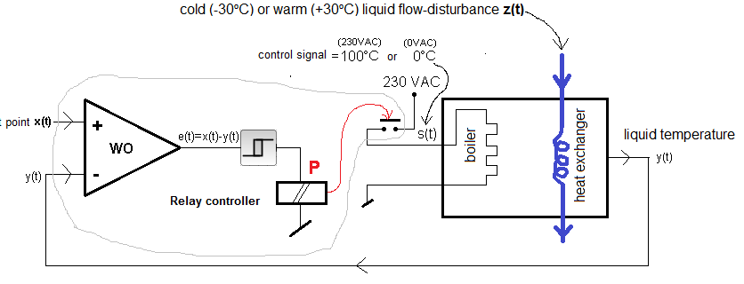

Fig. 21-17
Control On-Off system with disturbances.
The main purpose of each control (not only On-Off) is disturbance suppression. Thanks to this, you have a constant temperature in the refrigerator in summer and winter. The automatic pilot guides you in a straight line regardless of wind disturbances, etc. Positive disturbance z(t)=+30°C and negative z(t)=-30°C have already been described in the previous chapter 21.6. We expect that despite the disturbances, the average outlet water temperature will not change.
Chapter 21.8.2 On-Off Control with z(t)=+30°C positive disturbance.
In 5 seconds, the temperature setpoint +50°C will appear, which will remain constant all the time. The disturbance z(t)=+30°C (hot flow through the spiral) will occur in 35 seconds. Will the positive disturbance be compensated by the power drop on the boiler?

Fig. 21-18
Up to 35 seconds there is no disturbance, i.e. the time chart is the same as in Fig. 21-5. In 35 seconds, a disturbance z(t)=+30°C occurred.
Further analysis is similar as without disturbance only:
– when turned ON, the temperature tends to +130°C=100°C+30°C (because the heater + exchanger works)
– when turned OFF, the temperature tends to +30°C (and not to the ambient temperature, because the exchanger is still operating)
So there are short switchings ON and long OFF of the heater. The average power delivered to the water was therefore reduced. Anyway, the hysteresis of the relay keeps the temperature in the same band -5 ° C … – + 5 ° C as before the disturbance.
Note
A system with z=+30°C disturbance  be treated as without disturbance, except that the power behind the relay is increased by +30°C.
i.e. instead
ON=+100°C is ON=+130°C
OFF=0°C is OFF=+30°C
Chapter 21.8.3 On-Off Control with z(t)=-30°C negative disturbance.
The scheme differs from the previous one only in the disturbance z(t).
Previously, there was heating with z(t)=+30ºC
Now there is cooling z(t)=-30ºC
Will the disturbance be compensated by the additional power on the boiler?

Fig. 21-19
Up to 35 seconds there is no disturbance, i.e. the time chart is the same as in Fig. 21-5. In 35 seconds, a disturbance z(t)=-30°C (cooling) occurred.
Further analysis is similar as without interference only:
– when turned on, the temperature tends to +70°C=100°C-30°C (because the boiler heats and the exchanger cools)
– when turned off, the temperature tends to -30°C (because it still cools the exchanger)
So there are long switchings ON and short OFF of the boiler. The average power delivered to the liquid was thus increased. And again, the hysteresis of the relay keeps the temperature in the same band +5°C…-+5°C as before the disturbance.

Chapter 21.9 On/Off Control-Conclusions
This is the easiest adjustment that works by. rules
output too small–> control MAX
output too large–> control MIN
We learned the basic concepts of automatics – setpoint, output signal, control error, control signal and disturbance. As in any Control System, the value of the output signal tends to the setpoint value. Even when there are disturbances.
If you finished learning about controllers today, treat other , e.g. PID, as ON-OFF ones! The most important effect of their operation is the same –> they suppress disturbance. Another thing is that The ON-OFF Control does it in a crude way. The symptoms are that the output signal y(t) constantly undulates with the amplitude the greater, the greater the more inertia and delay of the object and the hysteresis of the controller. The other thing is that in many situations it doesn’t bother us. In the refrigerator, these temperature fluctuations are single Celsiuses. Ham, eggs and tomatoes won’t even feel it.