Automatics

Chapter. 20 Hurwitz Stability Criterion
Chapter. 20.1 Introduction
The Nyquist, known earlier, was an example of a frequency-type stability criterion. I don’t think I need to explain why. The second approach is the analysis of the transmittance G(s). The problem is related to the study of the equation M(s)=0, where the polynomial M(s) is the denominator of the transmittance G(s)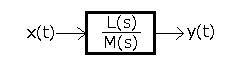

Fig. 20-1
G(s) as a fraction.
Conclusion
The automatics engineer should be well versed in M(s)=0 type equations. When M(s) is, for example, a degree 5 polynomial, then the equation M(s)=0 can be, for example.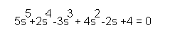

Fig. 20-2
An example of a degree 5 equation.

Chapter. 20.2 Quadratic and higher equations and complex numbers
We are well acquainted with equations of the 2nd degree, i.e. quadratic, not to mention equations of the 1st degree. There are also formulas for the roots of equations of degree 3, maybe even 4. Above, there are no such formulas. Or they are, just waiting for their Columbus. By the way, maybe someone knows the exact degree of the equation for which there is no longer a formula? I will be grateful for your response. In any case, equations of higher degrees can only be solved numerically – that is, by approximation. Let me remind you of the well-known formula for a quadratic equation.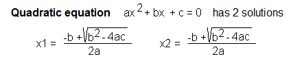

Fig. 20-3

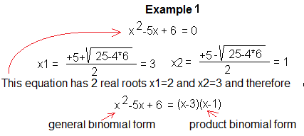
Fig. 20-4
Here Δ is non-negative and therefore the equation has 2 real roots x1=3 and x2=2. Knowing the roots of the quadratic equation, we can also write the product form of the binomial. It is comfortable because you can see the roots in it. Let’s solve one more equation.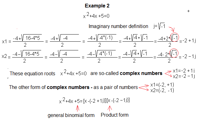

Fig. 20-5
Negative delta! In high school we would say “the equation has no solutions”. However, if we assume that there is such a strange number j that its square is -1, (or is equal to the root of –1, i.e. √-1), then there are 2 roots: x1=-2+1*j and x2=- 2-1*j. In this way, we entered the country of complex numbers.
Where does that name come from? Because they form a set of two numbers. The first is the real part, the second is the imaginary part. You have been using complex numbers since the first grade of primary school. What you didn’t know was, that you only used the real part of this number. The imaginary part was always zero. Therefore, when buying 3 kg or (3.0) kg of potatoes, you will always get the same thing. The second time you treated (3.0) kg or otherwise (3+j*0)kg as a complex number.
A side note.
For mathematicians, an imaginary number is i. Electricians fell in love with complex numbers at first sight, especially when alternating current, i.e. sinusoids shifted in phase, appeared. From the previous chapter, you know that these sine waves are beautifully presented as vectors. Then, for example, the sum of 2 sinusoids is easily represented as a vectors sum. Not only that, differentiating or integrating sinusoids is simply shifting them by an angle of +90° or -90°. For vectors, it’s a banality. And a vector is almost a complex number!
Returning to mathematicians and electricians, the latter use the symbol j instead of i. The justification is simple.
The i symbol would clash too much with the current symbol.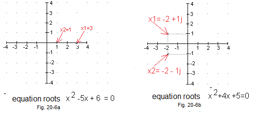

Fig. 20-6
Geometric interpretation of complex numbers as equations roots.
Fig. 20-6a
Equations roots as real numbers x1=3 and x2=1 (They are complex numbers too!)
Fig. 20-6b
Equations roots as complex  numbers x1=-2+1j and x2=-2-1j

Polynomial as a product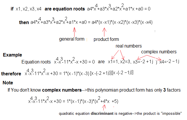

Fig. 20-7
How to factorize a degree 4 polynomial?
It is enough to know its 4 roots-> x1, x2, x3 and x4. These can be real or complex numbers. The methods for higher degrees 5…n are analogous. There are no general formulas for roots when M(s) is of high degree. Numerical methods of limited accuracy are then used.

Chapter 20.3 Roots of the denominator M(s) of trasmittance G(s) real only – What stability?
It will turn out that the denominator of the transmittance G(s) determines the stability.
Chapter 20.3.1 Stable-All roots of the denominator negative

Fig. 20-8
We study the transmittance G(s), whose denominator is a polynomial of degree 2 M(s)=s²+4s+3. The top is the same G(s), but the denominator is a product. You can check. And why in the form of a product? Because it shows the roots s1=-3 and s2=-1 of the quadratic equation M(s)=0. Both are negative. Well, so what? The Dirac impulse brought the system out of equilibrium, but after about 3 seconds it returned to equilibrium. In addition, without any adjustments. i.e. the course of y(t) was positive all the time.

Chapter 20.3.2 Unstable – the positive root of the denominator appears
Here one positive root s2=+0.075

Fig. 20-9
As expected, the system is unstable. The output of y(t) tends to + ∞. This was caused by the positive root of the denominator s2=+0.075.
We examined 2 transmittances G(s) (Fig. 20-8 and 20-9) whose denominator M(s) had real roots. Or in other words, the Δ of the denominator was not negative. Even just one positive root is instability! This can be generalized to M(s) of any nth degree.
Conclusion:
G(s) is stable when all roots of the denominator M(s)=0 are negative.
And when the Δ is negative, that is, when the roots are complex numbers?

Chapter 20.4 Roots of the denominator M(s) of G(s) transmittance are complex numbers- What stability?
Chapter 20.4.1 Stable-All roots of the denominator have a negative real part

Fig. 20-10
Negative Δ–> the complex roots of M(s)=0 will appear. You can calculate similarly as in Fig. 20-5. The real parts of these roots are negative -1.  After a few seconds from the dirac impulse, the system returned to equilibrium. However, unlike Fig. 20-8, this return occurred with oscillations. Now we can modify the stability theorem we learned earlier.
The transmittance G(s) is stable when all the real parts of the roots of M(s)=0 are negative
The expression “real parts” refers to elements that are complex numbers and have a non-zero imaginary part. Therefore, the above theorem is a generalization of the previous theorem. M(s) polynomials are of course of any degree.
You can also add how the stability in Fig. 20-8 differs from the stability in Fig. 23-10:
–Fig. 20-8 – Return to equilibrium without oscillation. Then the roots are real numbers.
–Fig. 23-10 – Return with oscillation. Then the roots are  complex numbers.

Chapter 20.4.2 Stable- Roots of the denominator have a positive real part
And when the real parts of complex roots are positive? Can you guess?

Fig. 20-11
The real parts of these roots with M(s)=0 are +0.05. They are positive.
As we assumed, the system is unstable. The amplitude of oscillations grows to infinity. The reason was a pair of complex roots with positive real parts.

Chapter 20.5 Hurwitz Criterion – You don’t need to know the M(s) roots to assess stability!
The transmittance G(s) of an open system (without negative feedback) is often in the product form, i.e. we know its roots. It is also stable. Including the transmittance G(s) in the negative feedback loop will change its value to Gz(s). As you can see in the figure below, the denominator M(s) is no longer in the product form. For M(s) second degree this is not a problem, but for higher degrees it is not so nice. Formulas, if they exist at all, are no longer as simple as for a quadratic equation.

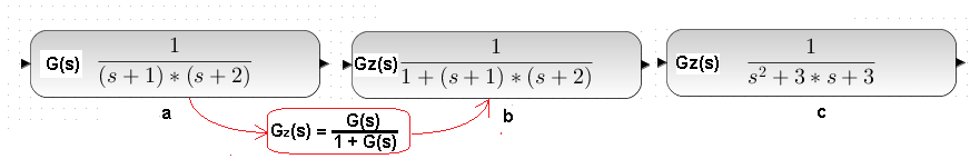
Fig. 20-12
-a In an open system, the denominator M(s)=(s+1)(s+2) is in the product form. The roots s1=-1, s2=-2 are visible. It is easy to judge that an open system is stable
-b closed system transmittance Gz(s) – intermediate result
-c transmittance of a closed system Gz(s) – the final result. Here M(s) is in the form of a polynomial. Roots are not visible.
You have to study the denominator of a closed system c. So it’s not like in Nyquist, in which you study an open system. Again, let me remind you of the stability theorem.
The transmittance G(s) is stable when all the real parts of the roots of M(s)=0 are negative.
Otherwise
The roots lie in the left half-plane of complex numbers, as, for example, in Fig. 20-6b. So you don’t need to know the exact values ​​of the roots. It is enough to know whether their real parts are negative. This is what the Hurwitz theorem deals with.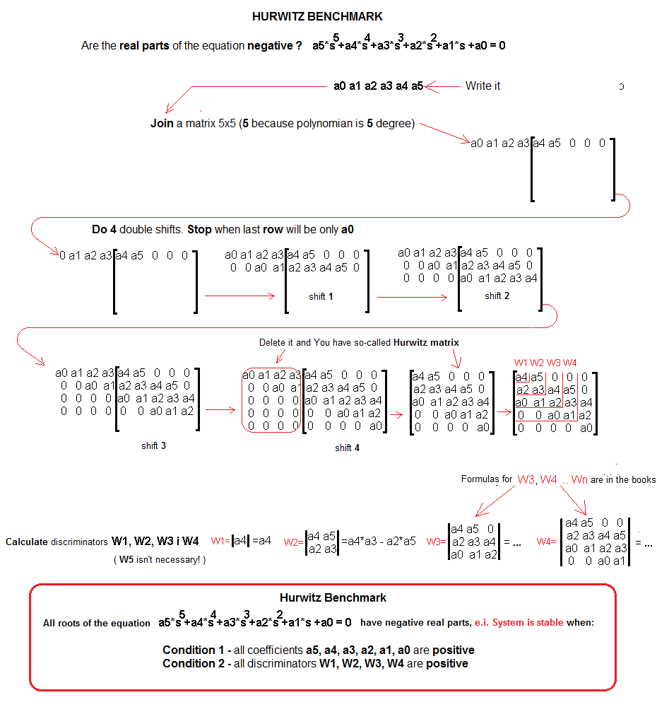

Fig. 20-13
This is what it looks like Hurwitz’s theorem for degree 5 polynomials. The mechanism for a polynomial of degree 6.7,…n works in a similar way.
I advise you to use this approach for all formulas “which, for any n”, are simply not very transparent. I personally check them for a specific n, as above for n=5. Then everything “sees better”.
If, Dear Reader, you are a high school student, you have the right to have a problem with W1, W2, W3 and W4 determinants.
Approach this hedgehog as follows:
– Each array (or matrix) of degree n is assigned a specific number called the determinant of degree n i.e. Wn
– The determinants W1 and W2 are calculated as in the above-mentioned drawing.
As for the next determinants, i.e. W3, W4, … Wn is a monkey job. They are given in every matrix calculus textbook.

Chapter 20.6. Checking the stability of the “stable” transmittance using the Hurwitz Criterion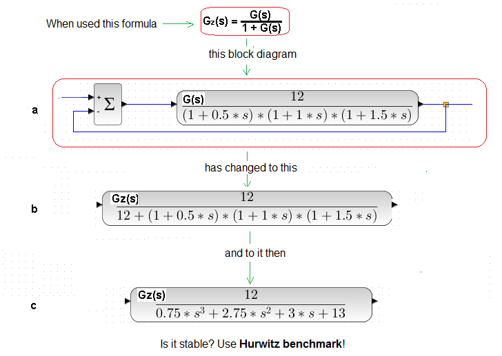

Fig. 20-14
On a we have the transmittance G(s) covered by negative feedback
On b we have the transmittance Gz(s) taking into account the negative feedback – immediately after applying the formula
On c we have the transmittance after the final transformations.
How to check the stability of Gz(s) using the Hurwitz criterion?
We remember that Mr. Hurwitz is only interested in the Gz(s) denominator.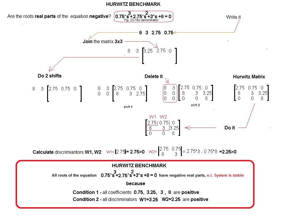

Fig. 20-15
It’s good that you don’t have to calculate the W3 determinant according to the 2nd Hurwitz condition, a little less work. Both Hurwitz conditions are met -> the real parts of the roots of the Gz(s) denominator in Fig. 20-15 are negative -> the transmittance is stable. How about we check? It is exactly Gz(s) from Fig. 20-14c. We will check the stability by tapping lightly with a dirac hammer. Will it return to a steady state, i.e. to y(t)=0, as promised by Hurwitz?

Fig. 20-16
It swinged and the system returned to a stable state where y(t)=0.
One more thing. Hurwitz says nothing about whether the roots of M(s)=0 are, real or complex. More precisely, do they have imaginary parts. From the oscillations it follows that some have. It also doesn’t say how stable the system is. How far from unstable.

Chapter 20.7 Checking the stability of the “unstable” transmittance using the Hurwitz Criterion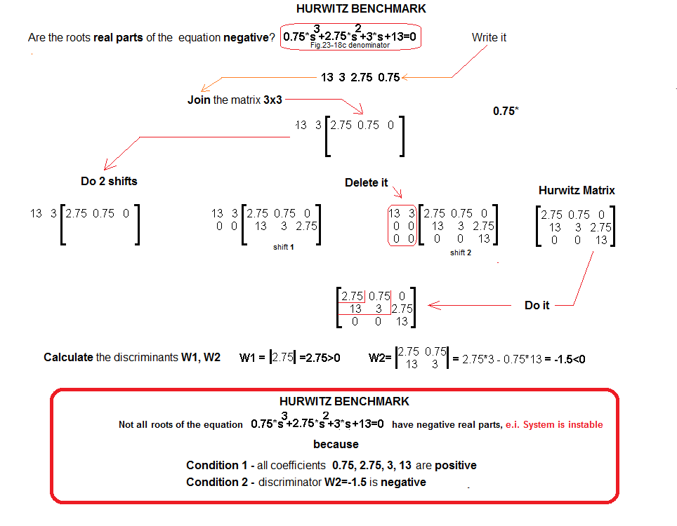

Fig. 20-17
On a we have the transmittance G(s) covered by negative feedback
On b we have the transmittance Gz(s) taking into account the negative feedback
On c we have the transmittance after the final transformations.
Similar to Fig. 20-15, we will check for stability.

Fig.20-18
Acc. Hurwitz. system is instable . We will check the stability by tapping lightly with a dirac hammer.

Fig. 20-19
System is instable! Hurwitz was right.