Automatics

Chapter 18. Amplitude-Phase Frequency Characteristics 
Chaptere 18.1 Introduction
You will learn the concept of amplitude-phase frequency characteristics in the most natural way. The input of the dynamic unit will be sinusoids with frequencies from 0 to infinity, and practically from very small to a specific large. The output sine wave will have the same frequency, but a different amplitude (usually lower) and a different phase (usually delayed) than the input one. The amplitude and phase of the open system determined in this way for the entire frequency range contain easy-to-read information about the stability of the closed system.
The frequency response of an open system is relatively easy to determine. You can do it “live” object in a facility without fear that you will lose control over the industrial installation. After all, it is an open system, and therefore stable.
If you know complex numbers, you will plot the amplitude-phase characteristic by substituting s=jω to G(s) and drawing successive values of the expression G(jω) for various ω pulsations on the complex plane.

Chapter 18.2 Rotating vector as a model of sinusoidal time charts
Cosines and sinusoids are often found in automatics, electrical engineering, acoustics…
Chapter 18.2.1 A rotating vector as a cosine 1cos(ωt)
We’ll start with the cosine.

Fig.18-1
Fig. 18-1a
cosine x(t)=1cos(ωt) for ω=1/sec as harmonic motion on the x axis
Fig. 18-1b
A rotating cosine of lenght 1 vector
A vector of length 1 has an initial state [1,0]=1+j0 and rotates at a rotational speed of ω=+1/sec (that is, with period T=2π sec and counter-clockwise). It is described by the complex equation z=1*exp(jωt)*
And now the most important! Projecting the end of the end of vector onto the x-axis is the animation in Fig. 18-1a!
Fig. 18-1c
Time chart x(t)=1cos(ωt)
The above 3 drawings describe the harmonic motion x(t)=1cos(ωt), which is exactly the same phenomenon. But the version of the rotating vector as z=1*exp(jωt) is the most intuitive model of the cosine function. Here the amplitudes A and the phase shifts φ are best visible!
*I suggest the chapter “Complex function exp(jωt)” as a rotating vector in the course “Rotating Fourier Series” chapter 2 in the Home Page with Courses. If you are less proficient with numbers and complex functions, take a look at the course “Complex Numbers”.

Fig. 18-2 
Rys. 18-2a
sine x(t)=1sin(ωt) for ω=1/sec as harmonic motion on the x axis
Fig. 18-2b
A rotating sine of lenght 1 vector
The vector has an initial state [0,-1] otherwise 0 -1j=-1j and rotates with a rotational speed of ω=1/sec
(i.e. with a period of T=2π sec.) It is described by the equation z=-1j*exp(jωt) or otherwise z=1*exp(jωt-90º). The projection of the end of  vector moves on the x-axis in Fig. 18-2a according to the equation x(t)=1sin(ωt).
Fig. 18-2c
time chart x(t)=1sin(ωt)=1cos(ωt-90º)
All this describes the harmonic motion x(t)=1sin(ωt). Note that the delay φ=-90º of sine 1sin(ωt) relative to 1cos(ωt) is best seen in the rotating vectors Fig. 18-2b and Fig. 18-1b.

Chapter 18.2.3 Rotating Delayed Cosine Vector 1cos(ωt-45º)

Fig.18-3
Fig. 18-3a
Cosine x(t)=1cos(ωt-45º) for ω=1/sec as harmonic motion on the x-axis.
Fig. 18-3b
Unit-vector rotation for x(t)=1cos(ωt-45º)
The vector has an initial state [1/√2,-1/√2] or 1/√2,-1j/√2 and rotates with a rotational speed of ω=1/sec (i.e. with a period of T=2π sec. ) It is described by the equation z=(-1/√2,-1j/√2)*exp(jωt) It can be described differently and probably simpler z=1*exp(jωt-45º). Its length (module) is 1. The projection of the end of the vector moves on the x-axis in Fig. 18-3a according to the equation x(t)=1(ωt-45º).
Fig. 18-3c
time chart x(t)=1cos(ωt-45º)

Chapter 18.2.4 Two rotating vectors 1cos(ωt) and 0.75cos(ωt-45º) i.e. with different amplitude and phase
We will meet with vectors of different amplitude and phase in chap. 18.5  and 18.6.

Fig. 18-4
Fig. 18-4a
Rotating vector z=1exp(jωt)
Fig. 18-4b
Rotating vector z=0.75exp(jωt-30º)
Fig. 18-4c
2 functions 1cos(ωt) and 0.75cos(ωt-30º)
Application
The vectors show the amplitudes and the delay ϕ=-30º cosine better than the time chart. Also remember that for full information, pulsation must be given with vectors – here ω=1/sec!

Chap. 18.3 Determination of the amplitude-phase characteristic of the proportional unit
We’ll start with the simplest dynamic unit . i.e. proportional.

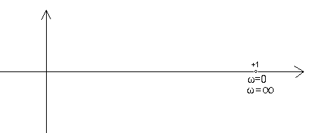
Fig. 18-5
Ampliltude-phase characteristic of the Proportional unit.
For this unit G(s)=1 at any time there is x(t)=y(t). So the output sine wave y(t) is equal to the input sine wave x(t) for each ω pulsation. Therefore, the amplitude-phase characteristic is so simple that it is difficult! It comes down to one point (+1.0).

Chap. 18.4 Determination of the amplitude-phase characteristics of the inertial unit.
Chap. 18.4.1 Introduction
So far, we mainly used time analysis of dynamic units. We gave as input x(t) unit step, Dirac impulse or sawtooth. Then the answer y(t) was information about the dynamic properties of this unit. I want the reader to associate the transmittance parameters G(s) with the appropriate time charts. Of course, knowledge of complex numbers will be useful for this, but it is not absolutely necessary. I just mentioned that s of G(s) is a complex number and not to worry too much about it. Therefore, one of the most basic concepts in automation has not appeared so far:
Amplitude-Phase Characteristics
It is an extension of the notion of frequency band. As input, we give a sine wave whose frequency slowly changes, theoretically from zero to infinity, and in practice it is only, for example, 30 frequencies from very small to high.
The answer y(t) is also a sine time chart with the same frequency, but with a different amplitude and phase.
These quantities, i.e. amplitude and phase, for different ω, shown in one diagram (e.g. Fig. 18-5), create an amplitude-phase characteristic. Unlike the “ordinary” band it also contains information about the phase of the sine signal.
We will now determine the amplitude-phase characteristic for the inertial term with the following parameters:
K=1
T=1 sec
We will start with a very small pulsation ω=0.31 1/sec (T=20 sec!) and end with ω=10.06 1/sec (T=0.63 sec). The green input sine wave x(t) always has a constant amplitude Xm=1. For each ω pulsation, we will determine the amplitude Ym and the phase φ of the red output signal y(t) in vector form.

Chapter 18.4.2 ω=0.31/sec (T=20 sec)

Fig. 18-6
The input is a green sine wave x(t) with an amplitude of Xm=1 and ω=0.31/sec (T=20 sec)
The output red sine wave y(t) has an amplitude Ym=0.95 and a delay φ=-17.5°. Sine wave y(t) is delaying behind by φ=-17.5° relative to the x(t). The same inusoids are also shown as vectors. The phase and the amplitude of the red sine wave y(t) are much better visible here. Parameters Ym and φ are determined as late as possible (here after about 25 seconds). Then the sine wave is already “calm down”. At the very beginning, we have a transition state in which the sine wave y(t) with the “elbow” is not really a sine wave yet. As you will see later, transients are more pronounced at higher frequencies.

Chapter 18.4.3 ω=0.63/sek (T=10 sek)

Fig.18-7
The input is a sine wave x(t) with amplitude Xm=1 and ω=0.63/sec (T=10 sec). The delay y(t) increased at φ=-32° and the amplitude decreased y(t) at Ym=0.85.
From the time chart, at first glance, it seems that ω is the same as before. But the time base has changed! Here and in the following experiments, the experiment lasts 30 seconds instead of 60 seconds as before.

Chapter 18.4.4 ω=1.26/sec (T=5 sek)

Fig. 18-8
Xm=1 and ω=1.26/sec (T=5 sec)
Delay y(t) increased at φ=-52° and the y(t) amplitude decreased  at Ym=0.61

Chapter. 18.4.5 ω=2.51/sek (T=2.5 sek)

Fig. 18-9
Xm=1 and ω=2.51/sec (T=2.5sec)
Delay y(t) increased at φ=-68° and the amplitude decreased y(t) at Ym=0.37

Chapter. 18.4.6 ω=5.03/sek (T=1.25 sek)

Fig. 18-10
The red arrow y(t) continues to delay and decrease. At higher frequencies, the transient state of the sine wave is more clearly visible at the beginning of the waveform.

Chapter. 18.4.7 ω=10.06/sek (T=0.63 sek)

Fig. 18-11
The red arrow y(t) continues to delay and decrease. At higher frequencies, the transient state of the sine wave is more clearly visible at the beginning of the red sine.
This completes the first stage of determining the amplitude-phase characteristics of the inertial unit 1/(1+sT).

Chap. 18.4.8 Amplitude-phase characteristics of the tested inertial unit
Let’s make one common drawing from successive phasor graphs (arrows).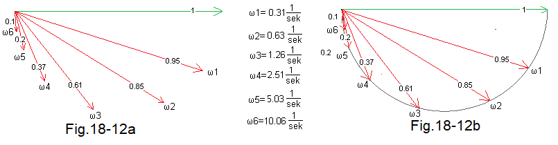

Fig. 18-12
A common drawing is Fig. 18-12a. The green vector is a symbol of 6 sinusoidal input signals x(t) with pulsations ω1…ω6 and amplitude Xm=1. The remaining 6 red vectors are the corresponding sinusoidal responses. There were only 6 pulsations here. What if there were more of them, e.g. a hundred, or let’s go all the way – a million? We will then obtain Fig. 18-2b, in which the end of the vector draws a semicircle.
Take another look at the next drawing.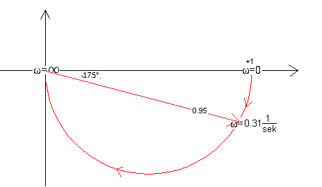

Fig. 18-13
The ends of all vectors are visible as a red semicircle. Added x,y axes. Seemingly similar, but how to treat the red response vector to a sinusoidal input signal x(t) with ω0=0 pulsation?
Firstly, we did not do such an experiment, and secondly, what is zero pulsation or frequency? Treat it as a very small pulsation! E.g. corresponding to the period T=1 year. All year you sit in front of the oscilloscope and watch the sine wave! You start on January 1 from the level x(t)=0. After the first quarter, you have a signal x(t)=+1, etc. You will agree that y(t) will also be slow and with almost zero shift φ. So small that you can take φ=0. The amplitude will also be 1.
Notice that we don’t have a green vector x(t). It was only needed for didactic reasons. Moreover, even red vectors are unnecessary. Here we have kept only one of their representatives for pulsations ω=0.31/sec. A semicircle alone is enough as the ends of various vectors.
The amplitude-phase characteristic is a generalization of the concept of frequency response (this, in turn, is a generalization of the concept of gain). From it, you can read not only the gain for a given pulsation, but also the phase. Here, for example, you can see that for ω=0.31/sec, the gain K=0.95 and the phase shift φ=-17.5°.
Each inertial unit with gain K=1 starts with pulsation ω=0 from the point (+1.0) and ends at ω=infinity at the point (0.0).
If the time constant T was twice as large, i.e. G(s)=1(1+2s), then for ω=0.31/sec there would be K=0.85 and φ=-32°.
For a different gain, e.g. for K=3, the beginning would be (+3.0) but the end would be the same -> also (0.0). The semicircle would be 3 times bigger.

Chap. 18.5 Determination of the amplitude-phase characteristic of the integral unit
Chap. 18.5.1 Integral unit as an example of astatic
The inertial and proportional unit are the so-called static units. They show the beginning for ω=0 and the end for ω=∞. And how it is for the astatic unit, e.g. integrating, you will see for yourself in a moment. We will study the integrating unit, similarly to the inertial unit.

Chapter 18.5.2 ω=0.31/sek (T=20 sek)

Fig.18-14
The output sine wave y(t) has an amplitude of 3.2 and a phase shift φ=-90°. Here’s a vector diagram of it that shows the same thing. The red output vector y(t) of length 3.2 is also delayed by φ=-90° relative to the input x(t).

Chapter 18.5.3 ω=0.63/sek (T=10 sek)

Fig. 18-15
The amplitude decreased twice to 1.6, but the phase φ=-90° remained the same!
Chapter. 18.5.4 ω=1.26/sek (T=5 sek)

Fig. 18-16
The amplitude decreased twice at 0.8, φ=-90°.

Chapter 18.5.5 ω=2.51 1/sek (T=2.5 sek)

Fig. 18-17
The amplitude decreased twice at 0.4, φ=-90

Chapter 18.5.6 ω=5.03/sek (T=1.25 sek)

Fig. 18-18
The amplitude decreased twice at 0.2, φ=-90°

Chapter 18.5.7 Amplitude-phase characteristics of the integral unit
Let’s make Fig.18-14…18 one common figure.

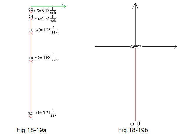
Fig. 18-19
The common one is Fig.18-19a.
Fig. 18-19b shows the amplitude-phase characteristic of the integral unit, without arrows and for all 0<ω<∞. For ω=0, the gain of the integrating term is K=∞ and for ω=∞, it is K=0.

Chapter 18.6 Static Units
They have no integrating elements. So they do not have single s in the denominator G(s). In response to a unit step, they give a steady state, and do not grow to infinity like astatic ones. It can be the previously presented inertial unit, as well as multi-inertial, oscillatory, delayed etc… Their characteristics, being more complex than inertial, are no longer semi-circles, but something similar. The three-inertial unit gives, for example, this characteristic.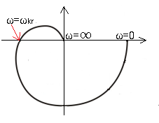

Fig. 18-20
The characteristics of the three-inertial unit pass through three quadrants. You can guess that two-inertial is only two quadrants, just like the poor thing, inertial only has one. For a certain pulsation ω=ωkr, the output sine wave y(t) of the three-inertial units is in antiphase to the input sine wave x(t) There is no such thing in the two-inertial term (because it is only in 2 quadrants), and even more so in the inertial unit.

Chapter 18.7 Conclusions
Previously, we treated the transfer function G(s):
-Intuitively as “something” that transforms the input signal x(t) output signal y(t). For example, the inertial term G(s)=2/(1+3s) transforms a unit step x(t)=1(t) into an exponential waveform y(t) tending to y=2 with a time constant of 3T. So you associated G(s) with the response to a unit step.
– Strictly as the quotient G(s)=Y(s)/X(s) where Y(s) is the Laplace transform of y(t) and X(s) is the Laplace transform of x(t).
It can be said that both definitions complement each other because:
-intuitive is not exact
-strict is not intuitive
Now the transmittance G(s) transforms each sine wave x(t)=1sin(ωt) with pulsation ω=0…∞ into a sine wave y(t)=Asin(ωt-φ) with amplitude A and phase shift -φ. An example is Fig.18-13. Here the inertial term G(s)=1/(1+1s) turns the input sine wave x(t)=1sin(ωt) for ω=0.31/sec into the output sine wave y(t)=sin(ωt-φ) where A =0.95 and φ=-17.5º. Each point of the amplitude-phase characteristic corresponds to the pulsation ω=0…∞, from which the amplitude and phase of the output sine wave y(t)=Asin(ωt-φ) can be read. In short, the transmittance G(s) is the phase-amplitude characteristic. It contains information on how to transform each input sine wave x(t)=1sin(ωt) in the range ω=0…∞ into an output sine wave y(t)=sin(ωt-φ). It is a generalization of the frequency response in which there is not only a gain K for each frequency, but also a phase shift -φ.
Note that the definition of G(s) as an amplitude-phase characteristic is quite strict and intuitive