Automatics
Chapter 17 Instability, or How Oscillations Are Created
Chapter 17.1 Introduction
The oscillations simply result from the solution of the differential equations describing the feedback dynamic unit. You will get a time charts that, in response to a unit step x(t), the output y(t) comes to a steady state y:
– without oscillations
– with fading oscillations
With certain parameters, including K gain, an unstable state with increasing oscillations may also arise.
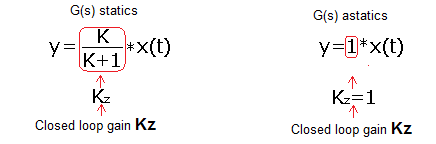
Fig. 17-1
Steady state y in a closed system when G(s) static or astatic.
In steady state, y(t)=y is constant. We call such systems stable. But that’s not always the case. With certain transmittance parameters G(s), especially with large K and large delays, y(t) oscillations of constant or increasing amplitude will occur. Then we deal with unstable systems.
Of course, you can stop at the fact that for some G(s) parameters the system is stable and for others unstable. These are the solutions of differential equations and that’s it. This approach, however, causes some unsatisfactoriness. Therefore, let’s try to analyze the problem common sense. We suspect that the oscillations result from the inertia of the system, from the fact that the response appears with a certain delay.
Example
You sail on a sailboat. It’s night, the wind is blowing and you’re heading for the lighthouse. For the sake of simplicity, let’s assume you only use the rudder. The control is simple. A small lighthouse to the right of your course, you counter the rudder to the left and vice versa. If there are no disturbances such as wind, waves, etc., you are sailing almost in a straight line towards the lighthouse. By the way. There is an integral relationship between the rudder and the course angle, which can reduce the error to zero. An experienced sailor sails in a straight line along an almost invisible hose. Now imagine that between the tiller (i.e. what you hold in your hand) and the rudder blade itself there is a delay element. How this device is built – it doesn’t matter. The important thing is that your hand movements are delayed, e.g. by To=10 seconds. A small gust of wind will change the course. You immediately counter. The effect will be visible only after To=10 sec. The boat start sailing no longer on a hose but on a large boa snake. With a large To, the course may even go completely apart. You will not the goal. We will draw an important and quite obvious conclusion from the voyage. Objects with large inertias and delays are more difficult to control. They can cause a hose, pardon the oscillations.
But let’s stop sailing and consider the operation of a pure delay term with K gain and feedback. In such a system, the generation of oscillations is the easiest to understand.
Chapter 17.2 Instability of the delay element with feedback
Chapter 17.2.1 Introduction
It is possible to analyze the system without using differential calculus. Calculate almost on fingers. We will come to an interesting conclusion, somewhat reminiscent of the Nyquist Criterion, which will be discussed in the next chapter.
An open system with a delay after closing with a negative feedback loop will be:
-stable when K<1
-unstable when K>1
-on the verge of stability when K=1
First we will examine the delay term itself. We’ve done it before, but it doesn’t hurt to do it again. Repetitio est mater studiorum.
Chap. 17.2.2 Study of the delay unit in an open system
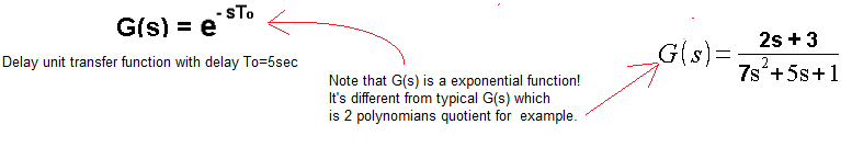
Fig. 17-2
Delay unit transmittance whose type clearly differs from typical G(s) transmittance.
Fig. 17-3
The response y(t) of the above delay unit G(s)=exp(-1s) is an exact copy of the input x(t) with a delay To=1 sec
Chapter 17.2.3 Delay unit in a closed system K=0.75 and To=1sec
Let’s close the delay unit with a negative feedback loop.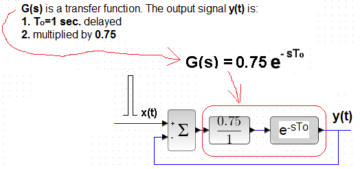
Fig.17-4
In front of the delay unit, an additional proportional unit was placed, whose gain K=0.75.
Fig.17-5
In 5 seconds, a rectangle pulse appears x(t)=1.
At this time, y(t)=0, therefore, at the G(s) input after the comparison node, there will also be the same rectangular pulse 0.75*x(t)=+0.75.
In 6 seconds
y(1) = 0.75*x(0) = +0.75
From 6 seconds, the comparison node only reverses the phase, because x(n)=0 and e(n)=x(n)-y(n)=-y(n).
The next signal after the delay element will be counted according to of the formula y(n+1)= – 0.75*y(n)
y(2) = – 0.75*y(1)= – 0.75*0.75= – 0.5625
y(3) = – 0.75*y(2)= + 0.422
y(4) = – 0.75*y(3) = – 0.316
y(5) = – 0.75*y(4)= + 0.237
y(6) = – 0.75*y(5) = – 0.180
y(7) = – 0.75*y(6)= + 0.133
y(8) = – 0.75*y(7) = – 0.100
y(9) = – 0.75*y(8)= + 0.075
e.t.c…
I emphasize that:
y(2) we calculated based on the known y(1),
y(3) we calculated based on the known y(2),
…e.t.c
This is the so-called recursive method.
Subsequent pulses y(n) are getting smaller and tend to zero. The impulse-type excitation threw the system out of balance and vanishing vibrations with a period of To=1 sec.
From a mathematical point of view, the sequence y(1), y(2), y(3), …, y(n) is a geometric progression in which:
y(1) = 0.75
The quotient of this progress q=- 0.75
Since |q|<1, the sequence tends to 0.
The tested transmittance was K=0.75<1. What if K=1?
Chapter 17.2.4 Delay unit in a closed system K=1 and To=1sec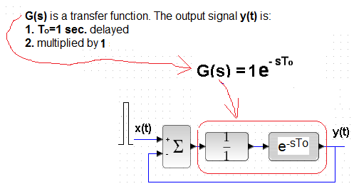
Fig. 17-6
In 5 seconds, a single pulse x(t) appears
Fig. 17-7
By analogy to Fig. 17-5:
y(1) = x(t) = +1
y(2) = -1*y(1) = – 1
y(3) = -1*y(2) = +1
y(4) = -1*y(3) = – 1
y(5) = -1*y(4) = +1
y(6) = -1*y(5) = – 1
…etc
The impulse also knocked the system out of balance, but this time it caused undying oscillations with a constant amplitude. The system has become a generator!
So for systems with a delay and gain K=1, the system is on the verge of stability.
What if K>1, e.g. K=1.25?
Chapter 17.2.4 Delay unit in a closed system K=1.25 and To=1sec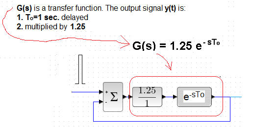
Fig. 17-8
In 5 seconds, a single pulse x(t) appears.
Fig. 17-9
The resulting oscillations whose amplitude tends to +/- infinity!
They had to be created because:
y(1) = 1.25*x(t) = + 1.250
y(2) = -1.25*y(1) = – 1.562
y(3) = -1.25*y(2) = + 1.953
y(4) = -1.25*y(3) = – 2.441
y(5) = -1.25*y(4) = + 3.051
y(6) = -1.25*y(5) = – 3.815
y(7) = -1.25*y(6) = + 4.768
y(8) = -1.25*y(7) = – 5.960
y(9) = -1.25*y(8) = + 7.451
…itd
Chapter 17.2.6 Conclusions![]()
Fig.17-10
If we enclose the delaying unit To in a negative feedback loop and give a signal to the input, e.g. a single pulse, the response will be oscillations about the period To and the amplitude:
-decreasing to 0..when k<1 –> stable system
-constant…………..when k=1 –> system on the verge of stability
-increasing ……… when k>1 —> unstable system
Note that based on the knowledge of the transmittance of the open system, we determined the stability of the closed system.
This is a bit like the Nyquist Criterion –> Chapter 18.
Chap. 17.3 Instability of the Three-inertial Unit with feedback
Chapter 17.3.1 Introduction
Previously, we studied the delay unit with negative feedback. It was so simple that we only used elementary mathematics and intuition. By increasing the gain K, the system became unstable. The source of this was the delay. This is also the case in continuous systems, but the concept of delay should be replaced with inertia. When there are many inertias T1, T2, T3, such as in the three-inertial unit, there will be something like a delay To. Then G(s) can be approximated by the equivalent transfer transmittance –> see Chapter 10.2.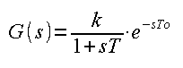
Fig. 17-11
Substitute Transmittance
For small T (not To!), the equivalent transmittance becomes similar to the ideal delay unit with k gain in Fig. 17-3. Let’s agree that when examining instability, the three-inertial unit is a representative of all continuous G(s) transmittances. A question may arise here. That’s why it’s not an even simpler two-inertial, oscillating or alone inertial unit. The analysis will be easier.
Well, as it turns out later, units with a monomial, a binomial in the denominator will always be stable! Even with a very large K. Yes, there will be oscillations, but they will disappear!
*assuming that the roots of the monomial or binomial are positive. But that’s usually the case in open systems.
Chapter 17.3.2 Test of the three-inertial unit in an open system
Fig. 17-12
Unstable systems can be stationary when input x(t)=0, like theoretically a pencil placed vertically on a table. Therefore, we will unbalance this and the next (especially) systems with the x(t)-“flick” signal. It is a short pulse with a duration of t=0.02 sec and an amplitude of 50. Its area is 1 and therefore we treat it as a approximation of the Dirac pulse. Remember about its large amplitude, especially since the oscilloscope “cuts” y(t) at +6 and -6 levels. The x(t) input acts on the trhree-inertial only for a short time from 3 sec to 3.02 sec. During this time, the energy from x(t) is stored in the unit, which then “discharges” giving such a y(t) waveform with a maximum for about t=5sec.
Compare with the response of the ideal delay unit in Fig. 17-3. You can see a certain analogy. Only that y(t) has been “blurred”. After some time t, the output y(t) reaches its maximum. This time is such a “pseudo delay”.
The analogy to the delay isn’t ideal, but the mechanisms causing instability in the ideal delay unit and the trhree-inertial unit are similar in feedback. For example, that increasing the K gain causes instability.
Rozdz. 17.3.3 Three-inertial unit in a closed system system K=3.
Fig.17-13
The input of the three-inertial unit is acted on by the signal e(t)=x(t)-y(t). At the beginning x(t) has a very large amplitude x(t)=50 but it works for a very short time 0.02 sec. Then all the time x(t)=0 and further increase of y(t) until reaching the maximum for t=4.3 sec is mainly due to the energy received from x(t) within 0.02 sec. Therefore, the initial time chart y(t) is similar to the open system in Fig. 17-13. Similar, but not quite. The maximum in the open system is slightly later, i.e. for t=5 sec. Why?
In the open system in Fig. 17-13, after 3.02 sec, the signal x(t)=0. The input signal on G(s) is zero and the time chart y(t) results only from the discharge of energy. However, in Fig. 17-13, the “braking force” e(t)=x(t)-y(t)=-y(t) is active all the time! This was not in Fig. 17-12. Therefore, the maximum occurred earlier, i.e. for t=4.35 sec. Nay! “Braking” –y(t) causes y(t) to reach the state y(t)=0 in 5.8 seconds and continue to run towards negative values. Now “braking” tries to turn y(t) back to y(t)=0. And so, with a few oscillations, the system returns to a steady state y(t)=0.
The study of the delay unit shows that by increasing K we can cause instability.
We expect that it is similar for the three-inertial unit as a representative of continuous objects (read “normal”). So let’s increase the gain from K=3 to K=7.
Chapter 17.3.4 Three-inertial unit in a closed system K=7
Fig. 17-14
The same rectangular pulse (“almost dirac”) x(t) is applied to the input.
The system swings longer, but is still stable. Greater rocking caused the larger K, which pushes y(t) more strongly in the direction of y(t)=0. That means more oscillations. Then let’s increase the gain to K=10.035. It will soon become clear why exactly 10.035.
Chapter 17.3.5 Three-inertial unit in a closed K=10.035
Fig.17-15
The system is on the verge of stability. For the delaying units, it was K=1, and here K=10.035, and there will be another value for the other dynamic units. The stability criterion is more complicated than for delay units. I guess it’s not surprising. After all, three-inertial is “more difficult” than delay unit. Now K=10.035 caused the next amplitude to have the same value as the previous one. If K were a little smaller, there would be no energy. The next amplitude will be a little smaller. When K is greater, the amplitudes will increase. Let’s check for, for example, K=12.
Chapter 17.3.6 Three-inertial unit in a closed K=12
Fig.17-16
The gain of K=12 is such that each subsequent amplitude gets a bigger kick. Amplitudes grow to infinity. The system is unstable.
Chapter 17.4 Three-inertial unit in a closed system – unit step x(t) as an input signal
Chapter 17.4.1 Introduction
When examining the instability, it was enough to “click” the dirac impulse on the three-inertial term to possibly bring it out of equilibrium y(t)=0. When the system was stable->Fig. 17-13, Fig. 17.14, it returned to the state of equilibrium y(t)=0. Otherwise, oscillations with a constant amplitude occurred–>Fig. 17.15 or increasing -> Fig. 17-16.
And how will a stable and unstable system behave when the input signal x(t) is a unit step of 1(t)?*
* more precisely, with a unit step x(t)=1(t-3) because it is delayed with respect to t=0 by 3 sec.
Chapter 17.4.2 Stable system unit step response
Fig. 17-17
Classic. The y(t) signal reaches a steady state y=0.75 acc. a well-known formula.
Chapter 17.4.3 Unstable system unit step response
It would seem that the steady-state Kz gain makes no sense for an unstable system.
It has a bit of that though.
Fig. 17-18
The oscillation amplitude increases to infinity around the constant component y=0.923 determined according to known formula.