Automatics

Chapter 12 Integration
Chapter 12.1 Introduction
There are indefinite and definite integrals.

Chapter 12.2 Indefinite integral F(t) from f(t)
The indefinite integral from the function f(t) is the so-called antiderivative function F(t) and is often simply called an integral.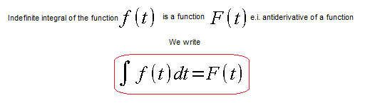

Fig. 12-1
The derivative of the antiderivative function F(t) is the function f(t) itself.

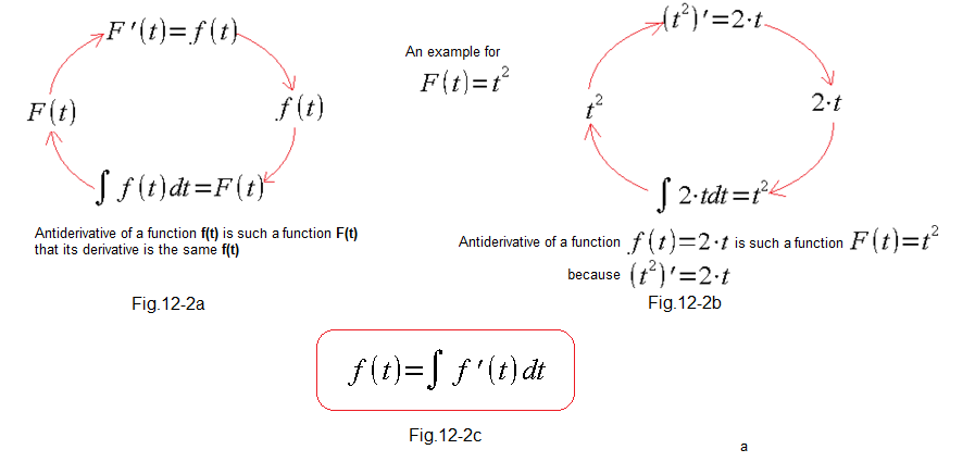
Fig. 12-2
Integration and Differentiation are mutually inverse operations. Integration as a calculation of the antiderivative function F(t) is a certain proficiency that first-year students of technical universities  acquire. It is needed to calculate the definite integrals. They will be discussed in a moment. Usually, in higher universities years, only the simplest integrals, otherwise, antiderivatives are remembered. This is the right approach, because you can always go back to your lecture notes.
In short soldier words. The antiderivative function from the derivative function is this function (Fig. 12-2c).

Chapter 12.3 The Definite Integral of x(t)
Chapter 12.3.1 Introduction
In automatics, we are dealing more with a definite integral than an indefinite one. The latter as an antiderivative function is used for very easy calculation of the definite integral value.

Chapter 12.3.2 The Definite Integral of x(t) as the area under x(t)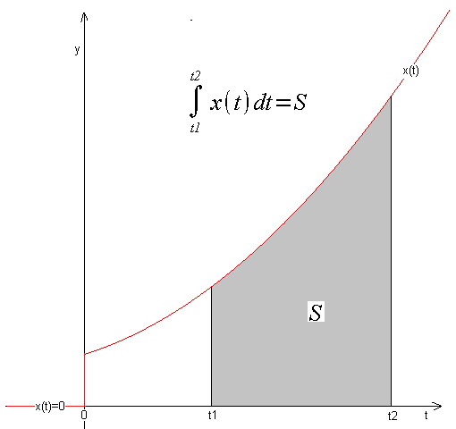

Fig. 12-3
The definite integral from t1 to t2 is the area S under the x(t) function. So it is a specific number, e.g. S=27.13. For our purposes, we will narrow this definition down a bit. In automatics, something usually starts at time t=0 and continues until time t. For example, the input signal x(t) can be a unit step or a saw. It is therefore assumed that for t<0 (negative!) the signal x(t)=0.–>Fig. 12-3.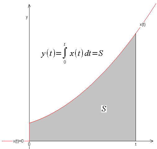

Fig. 12-4
So this is the version from Fig. 12-3 where t1=0 and t2=t. With this approach, the definite integral becomes a function y(t) and not a specific number.
And now the most important. How we calculate the fields in Fig. 12-3 and Fig. 12-4.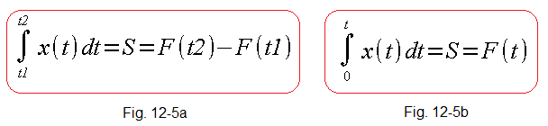 

Fig. 12-5
F(t1) and F(t2) in Fig. 12-5a are the values ​​of the antiderivative functions, i.e. indefinite integrals for t1 and t2.
We can also treat F(t1) itself as a area to the left of t1 and, analogously, F(t2) as a area to the left of t2. With this approach, the formula in Fig. 12-5a as the areas difference is obvious.
And in Fig. 12-5b, F(t) itself is simply an antiderivative! In the next 2 experiments, we will check if this is the case. Does the theory match the practice?

Chapter 12.3.3 The Definite integral of a Function that is a unit step x(t)=1(t)
Why exactly a unit step x(t)=1(t)? Because there is no simpler function and it is easy to calculate the definite integral=area S.
Let’s treat the definite integral as the output y(t) of the integrating unit whose input is x(t)=1(t). It turns out that y(t)=t(t)<–linear function

Fig. 12-6
The input of the integral unit is a unit step x(t)=1(t) and its output is the integral y(t)=t(t)
I remind you that:
1(t)=0 for t<0 and 1(t)=1 for t>0
t(t)=0 for t<0 and t(t)=t for t>0, i.e. t(t) is the so-called saw.
The integral from 0 to t of any function is the area under the graph of this function.
Here x(t)=1(t) is very simple and it is easy to calculate the area under the function as the area of ​​a rectangle with sides h=1 and t. For any t>0, the area y(t)=t(t)=t.
E.g. for t=5 y(t)=5. So theory matches practice.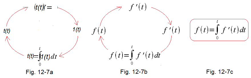

Fig. 12-7
So in short “the derivative of the definite integral in the range 0…t is an integrand function.
Fig. 12-7a
[t(t)]’=1(t) , i.e. the derivative of the integral is an integrand function
Fig. 12-7b
Generalization of the previous one
Instead of the function t(t) there is just a general f(t)
Fig. 12-7c
Ultimately
The definite integral of the derivative, which is f'(t) is a function of f(t). So differentiation is the inverse of integration.

Chapter 12.3.4 The Definite Integral of a function that is a saw x(t)=0.2*t
For the saw, the Definite Integral can be computed as the area of ​​a triangle. So let’s check if the output of the integral unit is a definite integral.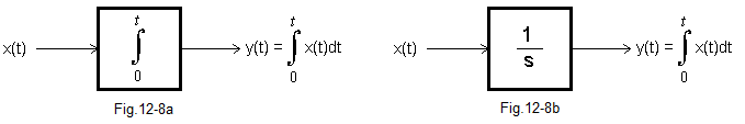

Fig. 12-8
The input of the integral unit is a “saw”, otherwise a linearly increasing signal, here according to the formula x(t)=0.2*t.
We will calculate the definite integral of x(t) as the area of ​​a triangle with base t and height x(t)=0.2*t.
Here, for example, for t=9sec, the saw x(t)=0.2*9=1.8 and the area of ​​the triangle S=0.1t²=8.1
Theory agrees with practice. The signal behind the integrating unit is a parabola with the given formula and for e.g. t=9 the output signal y(t)=8.1.

Chapter 12.3.5 The definite integral of the “slider swing” function. Otherwise type I manual control
The definite integral is always the area under the function from time t=0 to time t. Even when the function is more complicated like below. The integral can be positive, zero, or negative.

Fig. 12-9
Observe the output signal y(t) depending on the changing position of the slider x(t).
You will find that:
– The more positive x(t), the faster y(t) grows
– The more negative x(t), the faster y(t) decreases
– x(t)=0 is stopping y(t) at the last level.
This makes us believe that x(t)=y'(t). Imprecisely speaking, but accurate “x(t) is the derivative of the integral” or “the circles in Fig. 12-7 are true”.
In my experiment, 52 seconds when y(t)=0, then the positive area x(t) is equal to the negative area (area counted up to t=52 sec.)

Chapter 12.4 Conclusion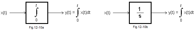

Fig. 12-10
Integral units symbols
Fig. 12-10a 
Using the integral symbol
Fig. 12-10b
Using operational calculus