Automatics
Chapter 11 Differentiation
Chapter 11.1 Introduction
If you know the topic, you can skip this chapter. But if not or “not very much”, then I heartily recommend it. So far, the most commonly used concept was Transmittance G(s), as “something” that connects the output y(t) with the input x(t). For systems devoid of dynamics (ideal amplifier, lever, toothed gear ….) it is simply the gain K, i.e. the proportional unit with the transmittance K.
At the first approach to a given phenomenon, technological process, almost everything is a proportional unit. You have an electric heater in your apartment, where the input x(t) is the power knob and the output y(t) is the temperature. You know from experience that if there is a constant temperature outside, e.g. –10ºC, the windows are closed …, then x(t)=1 kW will cause the temperature in the room =+20ºC, x(t)=1.1kW–>=+21ºC, x( t)=1.2kW–>=+22ºC…etc. You treat the entire system with the furnace and the room as a proportional unit.
After some time, however, it will matter that the temperature increase, e.g. by ΔT+5ºC, will last about 20 minutes. It is already a dynamic object for you. Quite simply described, but always there. Then you will approximate this system with the inertial unit. Then, more precisely, as inertia with delay, i.e. Substitute Transmittance. Perhaps it will be possible to identify the object as four-inertial, which has 4 time constants T1, T2, T3, T4 and gain K.
So far, you’ve treated the transfer function G(s) as “something”, which gives the appropriate output signal y(t) to the input x(t) – most often a unit step. You also know what a small lonely letter s in the denominator G2(s) can cause compared to G1(s), not to mention the letter s in the numerator G3(s).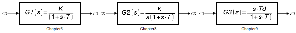
Fig. 11-1
If you don’t know, then quickly return to the relevant chapters.
After reading chapters 11…15, you will have an initial idea about:
– Derivative
– Definite Integral
– Differential equations, including linear differential equations on which the control theory is based
– Operational Calculus as a tool for solving linear differential equations
– Transmittance G(s) as an equivalent of a differential equation describing a dynamic object.
Chapter 11.2 The Derivative of a function
I repeated ad nauseam, especially in chapter 5, that the derivative of a function is the “speed of the function”!!! If you don’t feel it, then repeat this chapter. For the derivative term G(s)=s*Td, the output y(t) is proportional to the derivative of the input x(t), i.e. to x'(t). And for Td=1 sec, the output y(t) is simply the derivative of the input x(t).
In mathematical analysis, there are formulas that assign a derivative to each function. Thus, the differentiator in Fig. 5-7 in Chapter 5 converts the square wave signal x(t) into a y(t)=2*t signal. If you feel like it, go back to this chapter and repeat the experience.
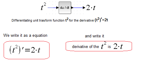
Fig. 11-2
Every 1st year polytechnic student starts mathematical analysis with these formulas.
Chapter 11.3. The second derivative, or “derivative of the derivative”
The derivative is a function. So you can recalculate the derivative, i.e. the second derivative, from this function.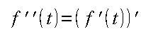
Fig. 11-3
On a specific example of f(t) as a square function, we will calculate the second derivative of this function.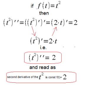
Fig. 11-4
Let’s check it by double differentiation.
Fig. 11-5
After the first differentiating unit we have the first derivative x'(t), and after the second – the derivative from the first derivative, i.e. the second derivative x”(t). Let’s check whether the theory agrees with practice.
Correct! If you don’t believe me, check with specific values.
If there was also a third differentiating unit, then we would get the third derivative or x”‘(t) as a derivative of the second derivative x”(t):
x”‘(t)=[(x”(t)]’ = (2)’ = 0 . The derivative of a constant function (2)’=0 is always zero because the “speed” or “slope” of a constant function is always o. The third derivative is the t (time) axis of the graph.