Automatics
Chapter 10 Delay Unit and Substitute Transmittance
Chapter 10.1 Delay Unit
Chapter 10.1.1 Introduction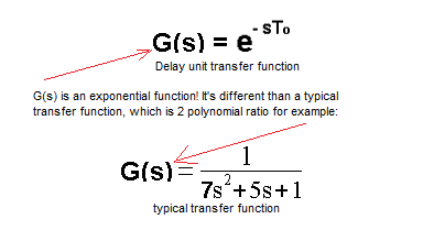
Fig. 10-1
Transmittance of the delay unit compared to typical transmittance.
The delay unit only delays the signal by To time without changing its shape. It’s hard to give an example. Maybe an echo? Or a conveyor belt on which sand is fed from somewhere out there. If the input is the sand level at the beginning of the conveyor belt, then at the end of the conveyor belt the level will be the same, but with a certain delay To.
Generally, almost every dynamic unit introduces some delay of the output signal relative to the input signal, but it is distorted by its inertia. On the other hand, the delaying unit is a pure delay. It is useful for creating substitute transmittance which the second part of the chapter concerns.
Chapter 10.1.2 Delay unit with slider and bargraph
It is a nasty dwarf that mimics you with a delay of To=5 sec
Fig. 10-2
The unit restores the state of the slider with a delay of To=5 sec. This can be seen in the movements of the slider and bargraph, as well as in the digital meters.
So its transmittance is:
Fig. 10-3
Typical transmittance is the fraction G(s)=L(s)/M(s), where L(s) and M(s) are polynomials. Only the delay unit as an exponential function, does not fall into this category! It looks pretty scary. Not only is it an exponential function, it’s also a complex number s in power. Don’t worry about it! Treat the delay unit as something that shifts the input signal by time, here To=5sec.
Chapter 10.1.3 Delay unit with slider and oscilloscope
The properties of the delay unit can be seen even better on the oscilloscope
Fig. 10-4
The output y(t) exactly reproduces the input x(t) from the slider with a delay To=5 sec. Nothing more to add.
Chap. 10.2 Substitute Transmittance
Chap. 10.2.1 Introduction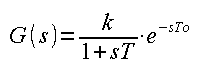
Fig. 10-5
The equivalent transmittance consists of an inertial and a delaying unit. Many commonly used dynamic members are multi-inertial, especially in the chemical industry. And these, in turn, can be approximated as equivalent transfer functions.
There are only 3 parameters in it:
k – steady-state gain
T – time constant of the inertial term
To – delay.
This is important for the optimal settings of the PID controller. There are formulas which for the object parameters k, T and To determine the optimal settings of Kp, Td and Ti of the PID controller. We will deal with this in chapter 28.
Let us remember that the equivalent transmittance is only an approximation of the real one.
Ch. 10.2.2 Determination of equivalent transmittance parameters based on the step response
Equivalent transmittance approximates multi-inertial unit. Let’s find it, for example, for the three-inertial unit. Usually, the determination of the parameters k, T1, T2 and T3 based on the response to the step is quite complicated.
Fig. 10-6
The animation shows how to replace the transfer function of the three-inertial unit with the equivalent transfer function based on the response to the step.
Draw a right triangle whose hypotenuse is tangent to the answer y(t) at its inflection point*. Determination of the normalized parameters T=6.2 sec and To=1.8 sec is obvious in the figure. The k=y/x=1 parameter is the gain in which y(t)=y=1, i.e. in a steady state after t=28sec.
What is this substitute transmittance for anyway? After all, the best approximation of the transmittance is itself.
Firstly
Often the object, which can be a tank in which something is mixed and chemical reactions take place, is not mathematically worked out. So I don’t know its transmittance. In contrast, designating a step response is easy.
Secondly
Even if we knew the transmittance of the object, it can be characterized by many parameters. One of the most important tasks of automation is the selection of appropriate controller settings. So that the response to the step was the most optimal in some respect. For example, the shortest control time with relatively small oscillations. This will be discussed in chapter 28.
Wise people have long worked out the selection of 3 settings of Kp, Ti, Td of the PID controller for various combinations of k, T, To of equivalent transmittance. Then they selected the appropriate tables for these 3 combinations – i.e. the appropriate equivalent transfer function. Our task is only to identify k, T, To as in Fig. 10-5 and select the controller parameters from the table.
Of course, you have to be aware that this is a rather “rough” method. After all, if we draw the tangent slightly differently, the parameters will be different. Especially The one that makes it extremely maliciously difficult to control.
In the next section, we will compare the response of the tested and substitute transmittance. Will the difference be big?
*inflection point of the function–> where the function “bends the other way”. The definition cries out to heaven for vengeance, but it couldn’t be simpler.
10.2.3 Comparison of test and substitute transmittance based on step response
Fig. 10-7
The unit step x(t) is fed to the input of the tested three-inertial unit and equivalent transmittance.
I didn’t expect the same answers. They differ, and quite a lot. Let us remember, however, that the parameters of the PID controller are ideally suited for the equivalent transmittance . And this means that the parameters of the PID controller for the tested transmittance, although not optimal, will be much better than if we tried to select them in a reasonable time by trial and error.