Fig. 2-1
Graph of f(x)=2x+1 and how to make it with Geogebra
After pressing the “triangle” of the video button, you will see the next stages of creating the graph.
1. I entered the text “geogebra.org” into any search engine, e.g. Google. Without the quotation marks, of course.
2. I pressed “Enter”.
3. I clicked the “Start Calculator” button
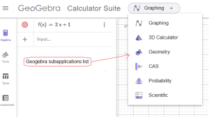
4. I am in the “Graphing” sub-application. I could already create the graph of f(x)=2x+1, but I will show the remaining sub-applications–> Fig. 1-2.
5. From the drop-down list, I selected the sub-applications “Graphing”, “3D Calculator”, “Geometry”, “CAS”, “Probability”, i.e. various branches of mathematics. The most frequently selected are “Graphing” concerning the function of one variable f(x). 3D graphics are functions of 2 variables f(x,y). CAS is like an enhanced version of “Graphing”, e.g. with differential calculus. “Probability” – the name itself suggests.
6. I finally returned to “Graphing”. Here in the “Enter…” window we entered 2x+1 and pressed Enter!, The program added “f(x)=” and a description of the graph f(x)=2x+1 was created. If you are a Doubting Thomas, check it out. For example, f(2)=5. That’s right. The point (2,5) lies on the graph.
Note:
The animation is a bit blurry. Maybe enlarging it will help? Press the square with the black diamond on the right end of the video recorder.

Fig. 2-2
Geogebra subapplications.

Chapter 2.2 Processing the graph of f(x)=2x+1.
You’ve already done the most important thing. You can draw the graph of f(x)=2x+1. That’s enough to study other functions, e.g. f(x)=x² or sin(x)…
But you can control the graph. Give it a function, choose the line color, line type – continuous or dashed, width, etc.

Fig.2-3
Final state of animation with graph settings.

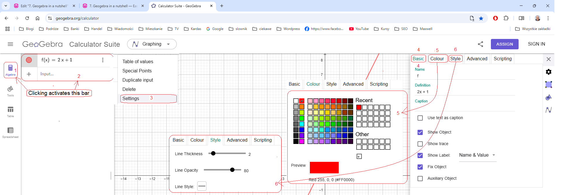
1. I click the “Algebra” button, which turns on/off the function entry bar.
2. I enter the function 2x+1 +Enter. The program will automatically add “f(x)=”.
3. I click the 3 vertical dots. A drop-down list of something opens, I select “Settings”.
4. The “Settings” window opens with the “Basic” tab. The other tabs are inactive.
5. In the “Settings” tab, you can change:
– function name – here f
– function definition – here 2x+1
– I recommend checking the “Show Object”, “Show Label”, “Fix object” boxes.
– in the “Name” box, I selected “Name &Value”.
5. In the “Color” tab, I select red.
6. In the “Style” tab, I select a solid line and a thickness of 3. You can select a dashed line and a different thickness.
7. I move the label and value, i.e. the text f(x)=2x+1, to a more visible place next to the chart.
I recommend playing around with the settings, also with other ones. Maybe it will be better. The animation should be enough. For complete clarity, I will also add a drawing with the windows that appeared in the animation.

Fig. 2-4
Graph settings windows that appeared in the animation Fig. 1-3

Chapter 2.3 What else should I set here?
In the animation I will show you how to:
1. Make a graph without a grid
2. Make a graph with a main grid (“sparse” grid)
3. Make it with a main and secondary grid
4. Enlarge and reduce the graph
5. Move the graph (left mouse button)
6. Return to the initial graph

Fig.2-5
Further processing of the f(x)=2x+1 graph.
It would be good if what is most important was more or less in the middle of the screen. The grid should also be optimal. Not too big, not too small.

Recognize operations 1…6 in the animation.

Chapter 2.4 System of 2 linear equations
Geogebra, or more precisely its “Graphing” sub-application , easily draws systems of 2 linear equations.

Fig.2-6
A system of 2 equations
x+y=4
2x-y=-1
After entering x+y=4, the name of the equation Eq1 was automatically added, and similarly for the second Eq2. I only set what was necessary. I skipped the colors, line thicknesses, etc. However, I selected the “name and value” label option. Thanks to this, the lines have the names Eq1: x+y=4 and Eq2:2x-y=-1. This greatly simplifies the analysis of the system of 2 equations. It doesn’t matter here, but in more complicated cases it does. The intersection of the lines gives the solution to the system of equations x=1 and y=3. Check it out..

Chapter 2.5 The graph of the function f(x)=x³-1.5x

Fig. 2-7
f(x)=x³-1.5x
Remember that the expression x³ is written like this–>x^3.
The label f(x)=x³-1.5x is covered by the VCR symbol. But it is visible for a moment during the animation.

Chapter 2.6 The graph of the function f(x)=xsin(x)

Fig. 2-8
f(x)=xsin(x)
A label with the name f(x)=xsin(x) is in the upper corner.
Notice how I change the gain of the graph to make it have a larger range.

Chapter 2.7 How to save, download and clear the graph?
I will show you how to download the Test graph file, view and clear it, create a new graph and save it as Test1. The files will be saved on your computer. You can also find it somewhere on the Internet, but we are not concerned with that for now.

Fig.2-9
How to save, download and clear the chart?
Note that the Test and Test1 files are already saved somewhere on the computer.
The animation will show:
1. Downloading the Test file
2. Viewing it as an x² chart
3. Clearing the screen with the x² chart
4. Creating a (x+3)(x-2) chart
5. Saving it somewhere as Test1. This file already existed, so it was only modified. You can of course save it as a new file with a new name