Scilab
Chapter 8. Function for solving Ordinary Differential Equations
Chapter 8.1 Introduction
This chapter is more about mathematics than Scilab. If everything is not clear, you can skip it.
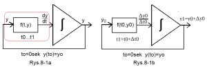
Fig.8-1
How does the integrator solve the first-order differential equation y'(t)=f(t,y)?
The system with an integrating unit solves the differential equation y'(t)=f(t,y) when initial conditions y(to)=yo. In other words, the entire differential equation is “enclosed” in the red box in Fig.8-1a. The comment will also apply to further diagrams with integrating circuits. Apparently it follows from the system itself, that at every moment t there is clearly y'(t)=f(t,y). Especially since the output of each integrating system is y(t) and the input is the derivative y'(t). But where is the beginning and end of events? A snake eating its own tail! Just some doubts. They should disappear when analyzing Fig.8-1b. At least here you can see what is the beginning. Namely, the initial state y(t0)=yo. So for to=0sec, there is a voltage yo at the output of the integrator. Most often, yo=0. Fig.8-1b shows, that for the initial state (to,yo) the difference quotient Δy0/Δto≈f(t0,yo) can be calculated, i.e. y1=y0+Δy0. And what’s next? We will again calculate the new Δy1/Δt1≈f(t1,y1), i.e. y2=y1+Δy1. Etc. This is how we will get the sequence of the output waveform y0,y1,y2…yn. This is an approximate solution to the differential equation dy/dt=f(t,y) with initial conditions y(to)=yo.
Note:
The analog circuit from the 1950s is the ancestor of the ODE function – a basic tool for solving first-order ordinary differential equations. And later, as it turns out, also of any order.
Section 8.2 Solving the y'(t)=1-y(t) equation using ODE
ODE – a function that solves arbitrary ordinary differential equation of first order
y'(t)=f(t,y)
at the initial conditions
y(to)=y(o)
This is a numerical implementation of the integrating system from Fig. 8-1 for any function f(t,y) with initial conditions y(to)=f(to).
The numerical solution for the specific function f(t,y)=1(t)-y(t) is given in Chapter. 7 in Fig.7-7 and this is implemented by program 7-2.
In a similar way, only for any f(t,y), the ODE function works.
Let’s check the operation of ODE for f(t,y)=1(t)-y(t) in the following program
P8-1 program with ODE function without comments
clc;
clear;
clf();
function ydash=f(t, y)
    ydash=1-y
endfunction
t=[0:0.1:10]
t0=0
y0=0
y=ode(y0,t0,t,f)
plot(t,y,'--or')
The same program with comments. Analyze it
clc;//Console cleaning
clear;//Data cleaning
clf();//Graph cleaning
function ydash=f(t, y)//Here starts ODE function as general ydash=f(t,y)
    ydash=1-y//Here is specific differential equation to solve
endfunction//Here ends ODE function
t=[0:0.1:10]//Time range
y0=0//initial state yo when t=0
y=ode(y0,t0,t,f)//ODE zalculates the solution based on to,yo
plot(t,y,'--or')//ODE creates graph y=f(t)
Note:
y’ is also known as ydash–>dash, an apostrophe after–>y a derivative symbol.
Execute program P8-1. The animation below will be helpful.
Fig.8-2
How to execute program P8-1?
You see the final animation result with the calculated y(t) graph, which is the solution to the differential equation y'(t)=1-y(t)
1. Place the Scilab Course and Scilab Console windows next to each other.
2. Call up the Scinotes editor (you have skipped the last edit file here)
3. Copy the P8-1 program from the Scilab course
4. Type P8-1 into the Scinotes editor
5. Execute wthout echo. Here Scilab tells you to save it somewhere.
6. Save the P8-1 program anywhere, under any name.
7. A graph of y(t) has been made as a solution to the equation y'(t)=1-y(t) with initial conditions y(0)=0.
The result is the graph in Fig. 8-2 whose “circles” correspond to the intervals Δ=0.1sec from the instruction t=[0:0.1:1].
I suggest you run the P8-1 program yourself. Just change the instruction plot(t,y,’–or’) to plot(t,y,’r’). Then the graph will be continuous.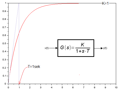
Fig. 8-3
Solving the differential equation y'(t)=1-y(t) as a graph of y(t).
In the next chapter you will learn that y(t) is the response of the inertial unit K=1 and T=1 sec to a unit step.
Chapter 8.3 Solving the differential equation y'(t)=1.5-2y*(t) using ODE
The flagship of the portal is Automatics, in which all experiments were performed in Scilab, or more precisely in its XCOS application. Another thing is that the reader is not dealing with Scilab here. And who has it? The author of the course who, for the convenience of readers, recorded animations of exercises performed with Scilab using ActivePresenter applicaton. Let’s go back to the Automatics course. At the beginning of the course you learn the so-called dynamic elements. Proportional, Inertial, Oscillatory... etc. Their dynamics is described by the so-called transmittance G(s). The inertial unit is shown below.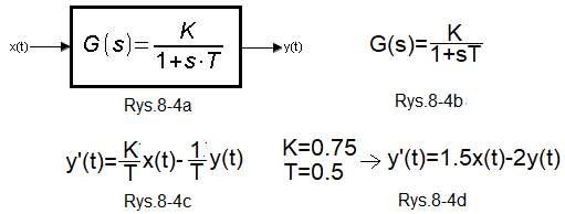
Fig. 8-4
Testing the Inertial Unit with the ODE function
Fig. 8-4a
Inertial Unit
Fig. 8-4b
Transmittance G(s) of the Inertial Unit
K gain
T time constant
Fig. 8-4c
Differential equation describing the transmittance of the Inertial Unit.
Note:
The relationship between the transmittance G(s) and the differential equation is shown in the course Automatics Chapter 15.3
Fig. 8-4d
Differential equation of the Inertial Unit for K=0.75 and T=0.5sec. When the input signal x(t) is a unit step 1(t), we will obtain the equation from the chapter title, i.e. y'(t)=1.5-2y*(t).
Let’s examine this unit with Scilab using the ODE function. The interpretation from the graph of the gain parameters K and the time constant T is obvious.
P8-2 program with ODE function
clc;
clear;
clf();

function ydash=f1(t, y)
    ydash=1.5-2*y
endfunction
t=[0:0.1:10]
t0=0
y0=0
y=ode(y0,t0,t,f1)
plot(t,y,)

t0=0
y0=0
y=1
plot(t,y,)
Description of the P8-2 program with the ODE function
How is it different from P8-1?
1. instruction ydash=1.5-2*y instead of ydash=1-y
2. plot(t,y,) instead of plot(t,y,’–or’) –> solid blue graph.
3. An additional sequence of instructions that plots the function y=1. This ensures that the graphs in Fig. 8-5 and Fig. 8-3 have the same scales.
t0=0
y0=0
y=1
plot(t,y,)
Execute program P8-3. You will get the graph in Fig. 8-5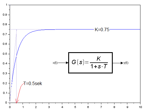
Fig. 8-5
Solving the differential equation y'(t)=1.5-2*y(t) as a graph of y(t).
Referring to Fig. 8-4, this is the response of the Inertial Unit with parameters K = 0.75 and T = 0.5 sec per step unit.
The interpretation of the K and T parameters is obvious. Look again at Fig. 8-3 with the Inertial Unit K=1 and T=1sec.
Chapter 8.4 Solving the differential equation y”(t)=0.5-0.125*y'(t)-0.25*y(t) using ODE
Section 8.4.1 General information about the above equation and its relationship to the Oscillation Unit.
As it turns out, we are dealing here with a response to a step unit of an Oscillation Unit with parameters K=2, T=2 sec and q=0.5.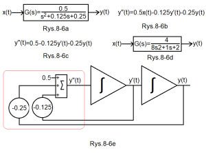
Fig.8-6
The Oscillation Unit and its differential equation
Fig.8-6a
Transmittance G(s) of this unit
At first glance it is not obvious that G(s) is an Oscillatory Unit. Or maybe it’s 2-Inertial Unit?
Fig.8-6b
The differential equation directly related to G(s) in Fig. 8-6a.
Even if you don’t know what transmittance is, try to find the dependence on G(s).
Fig.8-6c.
The differential equation when x(t) is step unit i.e. x(t)=1(t). So 0.5x(t)=0.5*1(t)=0.5.
Because 1(t)=0 for t<0 and 1 for t>1, and the range of the equation is for t>0.
Fig.8-6d
Exactly the same transmittance as Fig.8-6a, only written differently.
But from it you can obtain the parameters of the oscillating element K = 2, T = 2 sec and q = 0.25.
See the Automatics Course, chapter 7 Fig. 7-3.
Fig.8-6e
A system with 2 Integrating Units describing the equation in Fig. 8-6c
Note that it solves the equation y”(t)=0.5-0.125y(t)-0.25y(t), similarly to the system with one Integrating Unit from Fig. 7-6 chapter. 7 solves the equation y'(t)=1(t)-y(t). The second-degree differential equation is also included in the red box, as in Fig.8-1a.
Chapter 8.4.2 How does ODE solve the equation y”(t)=0.5-0.125*y(t)-0.25*y(t)?
I will not analyze in detail how to approximately solve the 2nd degree ordinary differential equation y”=x(t)-a*y'(t)-b*y(t). Or more generally y”(t)=f[t ,y'(t),y(t)] .
For the first degree equation y'(t)=f[t,y(t)] we replaced it with the approximate difference equation Δy/Δt=f[t,y(t)] with initial conditions y(to)=yo and then:
Δyo/Δt=f(to,yo) –>Δyo=f(to,yo)Δt
So we will calculate y1=y0+Δyo=y0+f(to,yo)Δt
Similarly, knowing y1, we will calculate y2 (because we will calculate Δy1/Δt1=f(t1,y1) etc…
That is
y2=y1+f(t1,y1)Δt
y3=y2+f(t2,y2)Δt
y4=y3+f(t3,y3)Δt
We assume that the time increments Δt are equal to –>Δt0=Δt2=Δt3=Δt4=…=Δt.
Note that based on the previous state y(n) we will calculate the next state y(n+1). This is the so-called recursive equation We know the first, initial state y(0)=yo.
The same will happen with the 2nd degree equation. But here we have 2 initial states, the function y(to) and its derivative y'(to). Here we will also replace the first derivative with the difference quotient Δyo/Δt=f(to,yo) and the second derivative (“derivative from derivative”) with the difference quotient (“increment from increment”) Δ(Δy/Δt)/Δt. Without going into details, this will lead us to a “double” recursive equation y(n+2)=f[y(n+1)] and y(n+1)=f[y(n)]. So, having 2 initial conditions y(to) and y'(to) we will calculate all y(2),y(3),y(4)…y(n),y(n+1). Wait a minute. Where’s y(0),y(1)? This can be easily calculated from the initial values y(to)=y(o) and y'(to)=y'(o). Conclusion, we will approximately solve a 2nd order differential equation.
Dear reader, maybe this is too general and you didn’t understand everything. Do not worry. This is a task for the ODE function. You just need to enter the appropriate parameters. But the most important thing is, that we will replace one second-order equation with two first-order equations.
Chapter 8.4.3 How does ODE treat the equation y”(t)=0.5-0.125*y(t)-0.25*y(t)?
First of all, it turns one second-degree differential equation into two first-degree equations. How? And as below.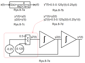
Fig.8-7
The oscillationunit and its differential equation as two first-degree equations
Fig.8-7a
Oscillation Unit
So Fig.8-6d is equivalent to Fig.8-6a
Fig.8-7b
Differential equation describing the Oscillation Unit
Fig.8-7c
As above but with two equations
Fig.8-7d
A version of two first-degree equations instead of one second-degree equation from Fig.8-7b
Fig.8-7e
An analog circuit with two integrators solving the differential circuit in Fig. 8-7d
I will add that it will give the same answer as the system in Fig. 8-6e, which is probably obvious.
Conclusion:
One second-degree differential equation can be converted into a system of two first-degree differential equations
General conclusion:
One third-degree differential equation can be converted into a system of three first-degree differential equations.
e.t.c…
And what about ODE?
P8-3 program
clc;
clear;
clf();
function ydash=f(t, y)
    ydash=[y(2);0.5-0.125*y(2)-0.25*y(1)]//after the symbol ";" we have entered the right side of the equation y2'(t)=...from Fig.8-7d
endfunction
t=[0:0.1:100]//range 0<t=<=100 with intervals Δt=0.1
t0=0//initial values t0=0sek
y0=[0;0]///initial values i.e. y2(0)=0 and y1(0)=0
y=ode(y0,t0,t,f)//function ODE call
plot(t,y(1,:))
xgrid(1,1,3)
Program P8-3 description
ydash=[y(2);0.5-0.125y(2)-0.25*y(1)]
This is a record of one second-degree differential equation with one unknown y(t) from Fig.8-7b in the version of two first-degree equations from Fig.8-7d.
Note:
In program P8-1 it was ydash=1-y. Are there any square bracket symbols here? Because they concern two variables y2(t) and y1(t) from Fig. 8-7c. Written as y1′(t) and y2′(t) from Fig. 8-7d.
That is, the vector [y1′(t),y2′(t)] or the vector [y(2);0.5-0.125y(2)-0.25*y(1)]. Here we marked y2(t) with the symbol y(2) and y1(t) with the symbol y(1). Do not associate it with any recursion!!!
Copy and execute this program in the Scinotes application as in the animation Fig.8-2.
You will get a chart like this.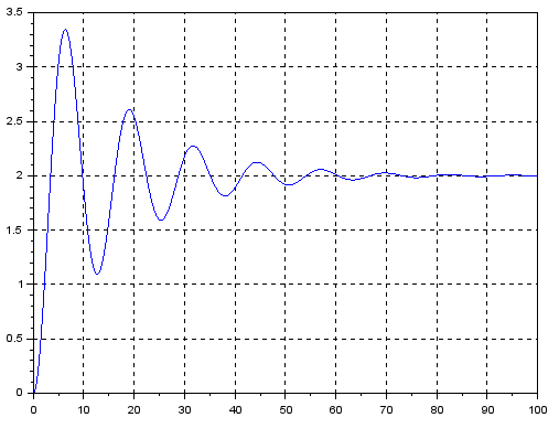
Fig. 8-8
Graph y(t) as a solution to the equation Fig.8-7b with initial conditions y(0)=0 and y'(0)
There may be some doubts about the derivative in Fig. 8-8. y'(0)≠0–>is not zero! ! Yes, but it should be y'(0)=0 with the note – for a homogeneous equation, i.e. for y'(t)=-0.125y'(t)-0.25y(t). And not the one with 0.5 as in Fig.8-7b.
Note:
You can read more about this oscillation unit in the course “Automatics” Chapter 7
Chapter 8.5 Solving the nonlinear differential equation y”(t)=0.5-0.125*y'(t)-0.25*√y(t) using ODE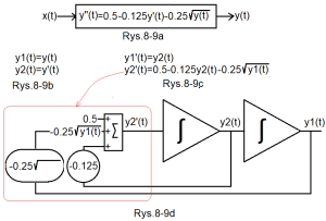
Fig.8-9
Nonlinear Oscillation Unit
Why non-linear? Because instead of 0.25*y (as in Fig. 8-7b), in Fig. 8-9a there is 0.25*√y (0.25*square root of y”)
Fig.8-9a
Due to non-linearity, the dynamic unit cannot be described as the transmittance G(s) as in Fig. 8-7a. But its dynamics more generally as a differential equation.
Fig.8-9b
The substitution is analogous to Fig. 8-7c. Nonlinearity doesn’t matter.
Fig.8-9c
Similar to Fig.8-7d
Fig.8-9d
Similar to Fig.8-7e. The difference is only in the root unit. The whole thing is solved by the differential equation from the title of the chapter.
The digital version of Fig.8-9d is the P8-4 program below with the ODE function. Comments are probably unnecessary here. The only difference is the root function sqrt(y(1)) used in ODE
Program P8-4
clc;
clear;
clf();
function ydash=f(t, y)
    ydash=[y(2);0.5-0.125*y(2)-0.25*sqrt(y(1))]
endfunction
t=[0:0.1:100]
t0=0
y0=[0;0]
y=ode(y0,t0,t,f)
plot(t,y(1,:))
xgrid(1,1,3)
Copy and execute it similarly to program P8-4.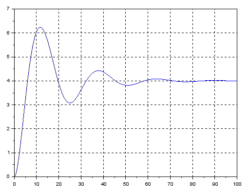
Fig. 8-10
Solution of a nonlinear differential equation
Compared to Fig.8-8, the response is more muted and lazy. This is the effect of signal square rooting.