Scilab
Chapter 7. Ordinary Differential Equations
Chapter 7.1 Introduction
Scilab is a specialized programming language for mathematical calculations. Mathematical operations, e.g. matrix operations, are much easier than in other languages. Therefore, he would not be himself, if he forgot about differential equations. More specifically about ordinary differential equations. This chapter will be less about Scilab itself and more about mathematics. You can skip it if you want, but I don’t recommend it. Scilab will only appear in the last section. Here we will solve the differential equation y'(t)=1-y(t) using the recursive method. They were also compared with the theoretical solution. The method of solving ordinary differential equations in Scilab works on a similar principle, only in a more sublime way. This is an ODE function, that we will discuss in Chapter 8.
Chapter 7.2 Charging a capacitor as an example of the simplest differential equation
That is, a first-order differential equation, i.e. the highest derivative in this equation is the first derivative dy/dt, or y'(t).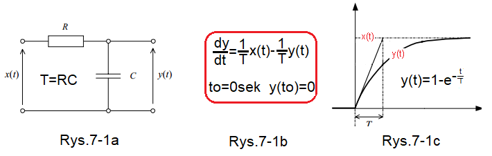
Fig. 7-1
Charging a capacitor as an example of a first-order ordinary differential equation.
Fig.7-1a
RC system
Every electrician/electronics engineer starts with this system.
Fig.7-1b
Differential equation describing the process of charging a capacitor.
The initial state, i.e. for to = 0 sec, the capacitor voltage y (to)=0V
The derivative y(t), i.e. dy/dt=(1/T)x(t)-(1/T)y(t), is the charging rate of capacitor C. It is the largest for to=0 sec, because capacitor C is uncharged (y( t)=0) and the difference (1/T)*x(t)-(1/T)*y(t) is the largest. Then the capacitor will charge a little and this difference will decrease. That is, the charging speed, otherwise the dy/dt slope will also decrease. Until we reach the steady state when dy/dt=0. Otherwise, y(t) will become a horizontal line.
Chapter 7.3 Generalization of a first-order differential equation.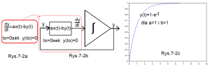
Fig.7-2
A more generalized differential equation
Fig. 7-2a
Generalization of the equation Fig.7-1a
This is an example of a first-order linear differential equation with the initial state to=0, y(to)=0.
Parameters a and b are arbitrary constants, e.g. a=1 b=1
Note:
I am an automation engineer and that is why I associate differential equations most often with time functions y(t), and less often with the shift function y(x). For a mathematician it has no meaning.
Fig. 7-2b
Diagram with an integrating system for solving the equation in Fig. 7-2a.
Back in the 1950s…1960s, computers were called analog and digital mathematical machines. Digital machines are simply computers, and analog machines are systems with integrating elements, somewhat forgotten nowadays, as above. In the red rectangle there is a diagram performing the mathematical operation ax(t)-by(t), or generally f(t,y). After the integrating circuit there is voltage y(t). In the initial state, to=0 often has the value y(to)=0. As for any integrating system, “after” is y(t), and “before” is the derivative dy/dt. The system will begin solving the differential equation starting from to = 0 and y(to) = 0, producing a waveform as shown in Figure 7-2c.
Fig. 7-2c
Solving the differential equation in Fig. 7-2a by the system in Fig. 7-2b.
a=1, b=1 y(to)=0 and when x(t)=1(t) is a unit step signal.
The analytical solution, or “pencil by a mathematician”, is y(t)=1-exp(-t). If you don’t believe it, substitute y(t)=1-exp(-t) into the differential equation y'(t)=1(t)-exp(-t).
Chapter 7.4 The most general first-order differential equation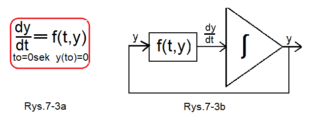
Fig.7-3a
The most general first-order differential equation
On the right side of dy/dt is an any expression f(t,y), where t is time and y is a function of time y(t).
In simple cases it may be e.g. f(t,y)=y(t).
Fig.7-3b
Diagram with an integrating system for solving the equation in Fig. 7-3a.
Chapter 7.5 Examples of first-order differential equations
The expression f(t,y) in the equation Fig. 7-3a is not very telling. Some specific examples will be useful
.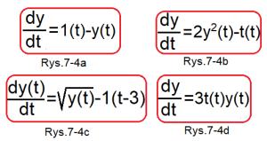
Fig.7-4a
First order linear differential equation
The signal x(t)=1(t) is a unit step, i.e. 1(t)=0 for t<0 and 1(t)=1 for t>0.
Here and in the remaining drawings I did not show the initial state, e.g. to=0 and y(to)=0.
Fig.7-4b
The differential equation is non-linear because it contains 2y²(t).
The function t(t) is the so-called “ramp”—>t(t)=0 for t<0 and t(t)=t for t>0.
Fig.7-4c
The differential equation is non-linear, because y(t) is “under the square root”. Signal 1(t-3) is a step delayed by 3 seconds.
Fig.7-4d
Another example of a nonlinear differential equation.
I will also add, that the input signal x(t) may be non-linear, e.g. x(t)=t²(t) or steps 1(t), 1(t-3), although e.g. dy/dt=3y(t)+t²(t) is a linear differential equation!
Chapter 7.6 How the model in Fig. 7-3b solves a differential equation?
We will analyze the system solving the differential equation in Fig. 7-3b. There, time worked continuosly. We will quantize it, i.e. we will examine its states in time up to t4 with a time interval of Δt. We know that the approximate value of the dy/dt derivative is the so-called difference quotient Δy/Δt. That is, dy/dt≈Δy/Δt.
It turns out that knowing the initial state y(to) we can calculate
Δyo/Δt=f(to,yo) –>Δyo=f(to,yo)Δt
So we will calculate y1=y0+Δyo=y0+f(to,yo)Δt
Similarly, knowing y1, we will calculate y2 (because we will calculate Δy1/Δt1=f(t1,y1) etc…
That is
y2=y1+f(t1,y1)Δt
y3=y2+f(t2,y2)Δt
y4=y3+f(t3,y3)Δt
We assume that the time increments Δt are equal to –>Δt0=Δt2=Δt3=Δt4=…=Δt.
In this way, we will calculate all values of y(ti) from the initial time to=0 to the final time here tk=10sec. So, knowing the initial state y(to)=yo, we will solve the first-order differential equation dy/dt=f(t,y). This is, of course, an approximate solution, the smaller Δt is, the more accurate it is.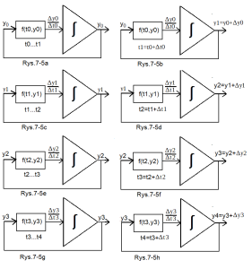
Fig.7-5
The state of the model in Fig.7-3a at time from t to t4
Fig. 7-5a
The output of the integrating element is the initial state y(to)=y0. The “pseudo-derivative”, or difference quotient Δyo/Δto=f(t0,y0) will be calculated immediately as a certain constant value. During the time Δto from to t1, the integrating unit “integrates” with the speed Δyo/Δto from the value y0 to y0+Δyo.
Fig. 7-5b
This is a photograph of Fig.7-5a at its final moment t1. So y1=y0+Δy0. This is also the initial state in Fig. 7-5c.
Fig. 7-5c
The initial moment t1 is the same as in Fig. 7-5b. This is actually the same state, except that at time t1 a new difference quotient Δy1/Δt1=f(t1,y1) is calculated as a new “pseudo-derivative”. During the time Δt1 from t1 to t2, the integrating unit “integrates” at the rate Δy1/Δt1 from the value y1 to y1+Δy1.
Fig. 7-5d
This is a photograph of Fig.7-5c at its final moment t2. So y2=y1+Δy1. This is also the initial state in Fig. 7-5e.
Fig. 7-5e
Description similar to Fig. 7-5c.
Fig. 7-5f
Description similar to Fig. 7-5d.
Fig. 7-5g
Description similar to Fig. 7-5e.
Fig. 7-5f
Description similar to Fig. 7-5d.
The next states for t5, t6, …tk are also calculated in a similar, i.e. recursive, way.
Chapter 7.7 How to solve a specific equation, e.g. dy/dt=y(t)-1(t)
That is, the solution for the equation in Fig. 7-4a as a special case in Fig. 7-2a, for a=1, b=1 and x(t)=1(t). The solution to this equation is Fig. 7-2c. Will the approximate solution based on Chapter 7.6 confirm this?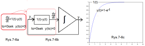
Fig.7-6
An integrator as a machine for solving the equation dy/dt=1(t)-y(t)
Fig.7-6a
Differential equation with zero initial conditions
Fig.7-6b
Integrator as a machine solving the equation dy/dt=1(t)-y(t)
Fig.7-6c
y(t)=1-exp(-t) as an exact solution (“in pencil”) of the equation dy/dt=1(t)-y(t)
I suggest substituting y(t) into the differential equation and checking. Remember that derivative [exp(-t)]’=-exp(-t)
Now we will solve this equation numerically, assuming dy/dt≈ Δy/Δt. The smaller the time increment Δt, the more precise it is.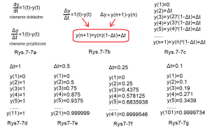
Fig.7-7
Numerical solutions of the differential equation y'(t)=1(t)-y(t)
Fig.7-7a
Exact differential equation–> y'(t)=1(t)-y(t)
Difference equation as approximate differential equation–>Δy/Δt=1(t)-y(t)
Fig.7-7b
How was the recursive equation y(n+1)=y(n)(1-Δt)+Δt obtained from the difference equation?
My grandson took his 8th grade exam yesterday. If the differential quotient were treated as an ordinary quotient, having nothing to do with differential calculus, it would arrive at the equation in the red box. Note that for a given increment of Δt, the coefficient (1-Δt) is constant, which makes the calculations very easy, e.g. for Δt=0.1 (1-Δt)=0.9.
Fig. 7-7c
The values of y(2),y(3),y(4)…y(n+1) calculated based on the equation Fig. 7-7b and the known values of y(1) and Δt.
y(1)=0 as the known initial value of the equation.
y(2)=Δt always
y(3)=y(2)*(1-Δt)+Δt is where the recursion begins.
Note that for a given Δt, e.g. Δt=0.1sec–>1-0.1=0.9, this recursion is very simple y(n)=y(n-1)*0.9+0.9
Fig. 7-7d
Next y(n) when Δt=1sec
Check for several n. Not very carefully, because Δt=1sec is large compared to the range t=10sec! If we increased e.g. Δt=2sec it would be even worse! Check. It goes with intuition. The smaller Δt, the more similar the difference quotient Δy/Δt is to the derivative dy/dt!
Fig. 7-7e
Next y(n) when Δt=0.5sec
Fig. 7-7f
Next y(n) when Δt=0.25sec
Fig. 7-7g
Next y(n) when Δt=0.1 sec
Conclusion
We expect that by decreasing Δt the response y(n) approaches the ideal solution Fig. 7-6c.
Chapter 7.8 Solving the above equation using Scilab.
Chapter 7.8.1 Analysis of the first part of the program
For now, we will analyze the first part of the program in which we will create and check the increase Δt of the difference quotient as well as the t vectors and the step unit.
7-1 program
clc;clear;clf
jtmax=10
Experiment_time=10
Δt=Experiment_time/jtmax
disp('Δt=',Δt)
t=0:1:jtmax
disp('t=',t)
step=t
for j=1:jtmax+1
   step(j)=1
end
disp('step=',step)
Let me remind you what each instruction does
clc;clear;clf
Standard cleaning of the console screen, variables and graphs
jtmax=10
The expected number of calculations here is 10, but in fact it will be jtmax + 1, i.e. 11.
Usually jtmax is larger, e.g. 100, 1000…
Experiment_time=10
Our differential equation covers time t=10 sec.
Otherwise, the domain of the differential equation is time t = 10 sec.
Δt=Experiment_time/jtmax
Δt time increment calculated for the difference quotient.
disp(‘Δt=’,Δt)
Δt display
t=0:1:jtmax
Vector t with discrete times t=[0,1…jtmax] on which the vectors will be defined
disp(‘t=’,t)
Display vector t
step=t
Definition of a new step vector. For now, the step is the same as t
for j=1:jtmax+1
step(j)=1
end
Conversion of the step vector from “time” to “step” (with “ones”). Here you may wonder why it is there
for j=1:jtmax+1 and not for j=0:jtmax? Because the vectors t and step do not start from t(0), step(0), but from t(1), step(1). Because that’s the typical of all vectors in Scilab.
disp(‘step=’,step)
step vector display
In the animation Fig. 4-2 in chapter 4 I showed how to execute the program in Scilab and there should be no problems with executing the above.
Follow this program. You will get something like this.
“Δt=”
1.// Since the experiment time t=10 sec and jtmax=10 then
Δt=1sec is quite large. Usually Δt is much smaller.
“t=”
0. 1. 2. 3. 4. 5. 6. 7. 8. 9. 10.
“step=”
1. 1. 1. 1. 1. 1. 1. 1. 1. 1. 1.
Everything, i.e. Δt and vectors, are as we predicted.
Chapter 7.8.2 Analysis of the entire program
Now that we have calculated jtmax based on it
-Δt – time increment
-t time vector with time units from 0 to 10 sec
-step vector with jtmax time units
then we can compare the differential solution y(j) from Fig. 7-7d…7-7g with the ideal solution from Fig. 7-6c on the graph. We expect that as Δt decreases, the differential solution will approach the ideal one.
Program 7-2
clc;clear;clf
jtmax=10
Experiment_time=10
Δt=Experiment_time/jtmax
t=0:1:jtmax
step=t
for j=1:jtmax+1
   step(j)=1
end//up to this point, description in chapter 7.8.1
ideal=step
for j=1:jtmax+1//see first explanation
ideal(j)=(1-exp((1-j)*Δt))
end
real=step
real(1)=0
for j=2:jtmax+1 //see second and third explanation
    real(j)=Δt+(1-Δt)*real(j-1)
end
plot(t,step,'o')
plot(t,step)
plot(t,ideal,'o')
plot(t,ideal)
plot(t,real,'o')
plot(t,real,'r')
The first explanation is when, for example, jtmax=10–>Δt=1sec
That is, we calculate the ideal graph of the solution of the equation in Fig. 7-6c for Δt = 1 sec
j=1–>ideal(1)=y(1)=1-exp(1-1)*1=0
j=2–>ideal(2)=y(2)=1-exp(1-2)*1=0.6321…
j=3–>ideal(3)=y(3)=1-exp(1-3)*1=0.8646…
j=4–>ideal(4)=y(4)=1-exp(1-4)*1=0.9502…
…
j=10–>ideal(10)=y(10)=1-exp(1-10)*1=0.9998…
We see that the calculations of the ideal solution coincide with Fig.7-1c
The second explanation when jtmax=10–>Δt=1sec
That is, we calculate the course of the approximate solution of the equation in Fig. 7-7d for Δt = 1 sec
j=1–>real(1)=y(1)=0
j=2–>real(2)=y(2)=Δt=1
j=3–>real(3)=y(3)=y(2)*(1-1)+Δt=Δt=1
j=4–>real(4)=y(4)=y(3)*(1-1)+Δt=Δt=1
…
j=11–>real(11)=y(11)=y(10)*(1-1)+Δt=Δt=1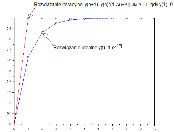
Fig.7-8
Graph of the ideal and iterative solution for Δt=1sec
The step unit 1(t) perfectly coincides with the “top” of the drawing. The iterative approximation is the upper dots and the lower ones are the perfect solution. You can see the difference between the ideal and iterative solution better than in the “numbers” in the first and second explanations. One more thing. In the graph, the circles were connected by straight lines, making the chart look like a real one.
Strange, the approximate course is almost rectangular. But this is the first and very rough approximation when Δt=1 sec. But if I hired a good lawyer, he would prove that an exponential chart is almost a step!
It will definitely be better when Δt=0.1. Let’s check
Third explanation when jtmax=100–>Δt=0.1 sec
That is, we calculate the chart of the actual solution of the equation in Fig. 7-7g for Δt = 0.1 sec
j=1–>real(1)=y(1)=0
j=2–>real(2)=y(2)=Δt=0.1–>=0.9
j=3–>real(3)=y(3)=y(2)*(1-01)=y(2)*0.9=0.1 9
j=4–>real(4)=y(4)=y(3)*0.9=0.271
j=5—>real(5)=y(5)=y(4)*0.9+Δt=Δt=0.3419
…
j=101–>real(101)=y(101)=y(100)*0.9+Δt=Δt=0.9999734…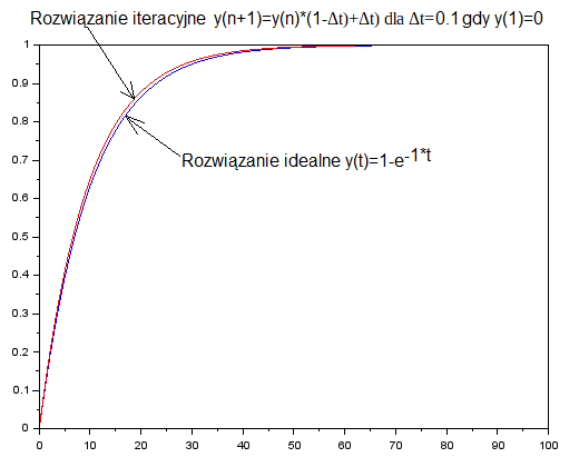
Fig.7-9
Graph of the ideal and iterative solution for Δt=0.1 sec
The chart is clearer because I gave up the dots. There would be 101 of them and it would make the chart less transparent. It is evident that the iterative graph came close to perfect. Let’s check this for jtmax = 250, when Δt = 0.04 sec. It will definitely be better, but by how much? We will give up the computational part and only provide a graph.
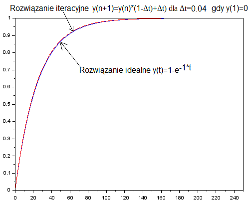
Fig.7-10
Graph of the ideal and iterative solution for Δt=0.04 sec
As we expected, the ideal graph almost coincides with the iterative one. It also coincides with intuition. The smaller Δt, the greater the accuracy of solving the differential equation. Will it be like this until the end? There are limits to reducing Δt. First, the computer itself calculates with finite accuracy. Secondly. The smaller Δt, the larger jtmax, the more iterations. And during iteration, errors accumulate. Maybe this will end our considerations about the accuracy of mathematical modeling. But we came to one basic conclusion. There is some optimal Δt. Not too big, not too small.