Scilab

Chapter 14 Xcos-Automatic Control Systems

Chapter 14.1 Introduction
XCOS is ideal for analyzing Automatic Control Systems.
First, we will examine the easiest to understand On-Off Control System. The controller is a relay with hysteresis, whose contacts control the electric heater of the furnace. The furnace will try to maintain the temperature within a certain constant range. At some point, the additional heater will turn on. The controller should reduce the power supply, so that the average temperature remains the same. This way you will learn the basic concepts of Control Theory. Set Point x(t) and disturbance z(t)–>switching on the additional heater. And ouput signal y(t)? What is his official name? This is a proces variable. 
Then we will deal with the P, I, PI and PID Control System. PID control is the most common type of control. For many PID controller is simply a controller

Ch. 14.2 On-Off Control Systems
Ch. 14.2.1 Relay with hysteresis
The animation will show how the relay works and what hysteresis is.
I usually encourage you to program the experiment yourself with XCOS, but here only animation analysis is enough.

Fig.14-1
Principle of operation of a relay with hysteresis.
A typical relay turns on, for example, at +5V and turns off, for example, at +4.8V. More useful in automation will be a relay characteristic that turns on at certain positive values and turns off at negative values. Here it turns on for x(t)=+0.2 and turns off when x(t)=-0.2. This creation must be supported by some simple electronics, the details of which we will not go into.
The signal inside the -0.2…+0.2 bar can change back and forth and does not affect the output signal. He may even go back to where he came from and return to the bar again “with impunity”. “With impunity”, i.e. without changing the relay state.
Chapter 14.2.2 On-Off Control System with positive disturbance z(t)=+30°C
The Object is a furnace as an Inertial Unit with T=15 sec. The relay turns on the power that would cause the temperature y(t)=+100ºC in the steady state. When turned off, the temperature y(t) approaches the ambient temperature, i.e. for example 0°C. In 5 seconds, the set point value x(t)=+50°C will appear, which will remain constant all the time. Disturbance z(t)=+30°C (switching on additional heater) will occur in 35 sec. Will a positive disturbance be compensated by an average power drop on the heater?

Fig. 14-2
At 35 seconds a disturbance occurred with z(t)=+30°C.
Further analysis is similar to that without disturbance, only:
– when turned on, the temperature quickly quickly strives for +130°C=100°C+30°C (because the additional heater is turned on)
– when turned off, the temperature slowly strives for+30°C (and not the ambient temperature, because the additional heater works)
So there are short switches on and long switches off of the heater. The average power delivered to the furnace was therefore reduced. Either way, the relay hysteresis keeps the temperature in the same range -5°C…-+5°C as before the disturbance.
Try to draw the diagram yourself in Xcos and press “Start”. The HYSTERESIS block can be found in the Discontinuities palette. You know the remaining blocks and know where to look. You can do it!

Chapter 14.3 Proportional Continuous Control System–>P contol
Chapter 14.3.1 Introduction
I hope you read chapter 13 carefully. The most important are the conclusions from the formulas in Fig. 13-5. Especially the fact that when the set point value x(t)=1(t), the steady-state output signal y=K*x/(1+K). E.g. for K=10 the output y=0.91. Generally, the larger K, the closer y approaches x. This will be the case for P type control. For I, PI and PID control it is even better. The steady output y will equal the set point value x. Regardless of any disturbances to the object! This is the main goal of Automatics.
Chapter 14.3.2 P Control without disturbance z(t)
By the way, we will compare the system without y1(t) control and with y2(t) control.

Fig.14-3
P control for the inertial unit – response to the unit step
You see 2 identical objects with output y1(t) and y2(t). And what’s that for? So that you can compare the same object in an open and closed system. The object with y2(t) is controlled by a P-type controller, whose only setting (parameter) is the gain Kp=10. After animation Fig. 14-3 and Fig. 13-3 and the formulas Fig. 13-5 from chapter 13, you will come to the conclusion that y2(t) reaches the steady state faster. True, it is y2=0.91x, not y2=x. So the error e=0.09 is not zero! However, in an open system, which is ovoid, the error e=0. This is the goal of every automatics engineer! Here, doubts may arise as to the closed system, which does not provide zero steady-state error e! They will disappear in the next subchapter.
Chapter 14.3.3 P control with disturbance z(t)=+0.2
The same object as before and with the same P controller when Kp=10. The only difference is the positive disturbance z(t)=+0.2, which will appear at 70 seconds. It’s as if you put an additional heater in the furnace, which in an open system would raise the furnace temperature by ΔT = +20ºC. The procedure takes 2 minutes, so please be patient.

Fig.14-4
 P Control-Response to unit step and disturbance z(t)=+0.2
The disturbance z(t) here is additional heating +0.2. As if an additional heater appeared or the voltage on the heater increased. Up to 70 sec. is as in Fig. 14-3. Per disturbance z(t)=+0.2 in 70 sec. the controller responded correctly. He lowered the heating power on the heater behind the controller. Although there is a slight effect of the disturbance, it was suppressed by a factor of 11. Complete damping, as you will see later, will only be provided by control with error integration e(t), i.e. type I, PI or PID.
Ch. 14.3.4 P Control-conclusions
1. Feedback improves the dynamics, the greater the Kp gain of the  P controller.
2. Remember the doubts from Chapter 14.2.2? The closed system improved the dynamics 11 times, but with a unit step it introduced a constant error of e=0.09. But it was 11 times smaller than without the controller!
3. Pay attention to the control signal s(t). Without disturbance and in the steady state, i.e. in the period 10…70 sec, the signal s(t)=y(t). This is typical for any P, I, PI and PID control. After 70 seconds, s(t) decreases, trying to compensate for the disturbance +z(t). Although it does not reduce the error to 0, it suppresses it significantly. This is typical of P regulation.
4. The P control responds quickly to input x(t), and quickly, although not completely, suppresses constant disturbances.
5. However, you would like to have a control, that brings the constant error e to zero.
Then read on.

Chapter 14.4 Continuous Control System I – only with integration
Chapter 14.4.1 Introduction
I controller is rarely used in practice. However, it is ideal for teaching purposes. You will understand the principle of feedback and disturbance suppression more easily than in the P controller. Especially since it can reduce the control error e to zero! This is why it is not used in practice. Because it’s beefy. I.e. it reaches a steady state very slowly
Chapter 14.4.2 The I controller test

Fig.14-5
Response to unit step of I controller  (integrating controller)
The most important element of each controller is the comparison node performing the subtraction e(t)=x(t)-y(t). Therefore, treat the signal x(t) in Fig. 14-5 as error e(t)! So we assumed that y(t)=0. A controller without a comparison node would be pointless. I controller has only one setting, integration time here Ti=2 sec. This is the time after which the output from the controller y(t) equals the unit step value x(t) at the input. Here after 2 seconds. That is, the larger Ti, the slower the signal from the I controller grows. Draw the I controller in Xcos and examine it with different x(t) amplitude values and different Ti settings.
Note:
The 1/2s integrating block will be obtained from the CLR block from the “Continuous-time systems” palette. Change the denominator from 1+s to 2*s
Chapter 14.4.3 I control with disturbance z(t)=+0.5
Again, you need to be patient. The graphs I type take a long time, here 4 minutes.

Fig.14-6
I controller-Response to unit step and disturbance z(t)=+0.5
Unlike P Control, in response to a unit step and a unit step disturbance, the control error in the steady state is zero, i.e. e=0. The response to a positive disturbance with z(t)=+0.2 is especially beautiful. When a disturbance occurs, y(t) tries to achieve y=1.5. But negative feedback reacts now. The integrating component will compensate for the disturbance until it does so completely when e=0. One could say that it will keep drilling a hole in belly…If the wonderful properties of the I component haven’t convinced you, Fig 25-6 in Chapter 25 of the “Automatics” course will do it.
Chapter 14.4.4 Conclusions
There is only one. In response to the x(t) unit step and z(t) disturbance, I control  reduces the error e to zero. However, it does it very slowly compared to P control Why? Compare the control response s(t) at the start with the kick in Fig. 14-4 and without the kick in Fig. 14-6. It is ,this kick that determines the dynamics. I like scientific language.

Chapter 14.5 PI-Proportional-Integral Continuous Control System.
Chapter 14.5.1 Introduction
P control gives a fast reaction, but a non-zero error. I control  the other way round, a slow reaction and a zero error. So let’s make a hybrid of these two controllers – a PI controller. We expect a fast reaction and zero error.
Chapter 14.5.2 Response of the PI controller to the unit step signal x(t).

Fig.14-7
Unit step response of the PI controller
Remember that, as in every controller, there must have a comparison node performing the operations e(t)=x(t)-y(t). For simplicity, we assume that y(t)=0 and therefore only examine x(t).
The PI controller has two settings
– gain Kp and doubling time Ti. We will calculate the Kp gain excluding the integration path.
Doubling time Ti 
– the time after which the controller’s output signal will double.
Or otherwise. The time after which the integrating component yi becomes equal to the proportional component yp.
Create the diagram with Xcos and play with the input x(t) and the Kp and Ti settings.
It will turn out that Kp and Ti do not depend on the unit step x(t).
Chapter 14.5.3 PI control with disturbance z(t)=+0.5

Fig.14-8
PI control – Response to unit step x(t) and disturbance z(t)=+0.5
Kp=10 and Ti=5sec were previously selected by trial and error method. They can be better. Try it.
Comparison with P-control in Fig. 14-4
The dynamics are similar, although there is a slight overshoot in response to the unit step. Better?, worse?
I don’t know. De gustibus non est disputantum. Let’s assume it’s neither worse nor better.
However, the error is zero.
Conclusion
PI control is better than P control
Now how does it work?
At the beginning of the set point  x(t) in starts in the 3rd second and the disturbance z(t) starts in the 70th second, the proportional component of the controller is mainly active. Therefore, the signal y(t) quickly approaches the steady-state value. This is, of course, not the value of the unit step  x(t), because P control will never ensure zero steady-state error e=0. This is the task of the integrating component. At first, its influence is not visible because the signal is only growing. It is visible later, when the P component ceases to have an influence. Then the integrating component, according to its role, will reduce the error to zero, i.e. e=0. This applies to the set point value x(t) and the disturbance unit step z(t). To sum up. The integrating component will continue to drill a hole in the belly until it brings the error e(t) to zero. Note that in the steady state the disturbance z(t)=+0.5 is compensated by the controller control signal Δs(t)=-0.5.
Chapter 14.5.4 Conclusions
1. The dynamics of PI control is comparable to P control.
2. PI control can reduce the control error to zero, which is not possible with P control.
3. The optimal Kp and Ti settings are those that will provide a relatively fast and overshoot-free y(t) signal in response to x(t) or z(t). It turns out that a “nice” answer to x(t) is often an “ugly” answer to z(t) and vice versa. The engineer role is to make the right choice. Depending on what appears more often. Change x(t) or disturbance z(t)? The note also applies to PD and PID control.

Chapter 14.6 Continuous PD Control System, i.e. Proportional-Derivative Control.
Chapter 14.6.1 Introduction
The derivative component responds to the speed of the input signal e(t). In the steady state there are no speeds, i.e. it gives a zero signal. This means that it is not able to eliminate the permanent error in e. However, it significantly improves the dynamics of the course.
Chapter 14.6.2 Testing the real derivative. That is derivative with inertia.

Fig.14-9
The response of the real derivative unit to a linearly increasing signal i.e “ramp”.
At some point, the input signal speed will double.
Think of the derivative unit as a speedometer with analog output, that measures speed with some inertia. The cheaper (worse), the greater the inertia. You can see how the output doubled when the speed doubled.
With inertia T=0.1 sec, of course. The signal stabilized after approximately 4T.
*We usually examine the response of the element to a unit step. But for the derivative element D, a signal that increases linearly, i.e. “ramp”, will be better. Why? Because with a unit step the speed of increase is infinitely high and this causes various problems.
How to calculate the parameters of this block. From the transmittance 1*s/(1+0.1*s) it is trivial to say that Td=1sec and T=0.1sec.
And from the chart? Just like in the animation. Of course, that’s right. Just remember that the intersection of the lines y(t) and x(t) is supposed to be for a steady y(t)!
Chapter 14.6.3 Response of the real PD controller to a linearly increasing signal.

Fig.14-10
Response to the linearly increasing signal (“ramp”) of the PD controller (with real differentiation)
Kp=1, Td=1sec, T=0.1sec
Why this real differentiation with inertia T=0.1 sec. I don’t think I’ve touched on this topic. Because ideal differentiation introduces “pins” in the case of quick changes in x(t), which adversely affects the regulation. The inertia T suppresses these disturbances. But let’s get back to the main story.
The “smoothing” after 1 and 5 seconds (then there is a change in the signal speed x(t) results from the fact that the real differentiation path needs about 0.5 seconds to “recover” and calculate the correct speed. In the steady state, the proportional components P and D are clearly visible, which is the same as for the ideal PD component. I emphasize – the same, but only in the steady state.
Note:
At first glance, it seems that the response to the increasing signal x(t) of the P and D components is similar.
But this only results from the fact that the control signal y(t) is a sum
–component P, which increases like Kp*x(t)
–component Kp*D which is almost constant. Apart from the initial inertia, of course.
Chapter 14.6.4 PD control with disturbance z(t)=+0.5
That is, with a huge disruption. It’s like putting an additional heater with half the power of the control heater into the furnace! The object will be double-inertial, not inertial as before. Why? Because inertial is an “easy” object to control. Just give a large Kp for the answer to be correct. In other words, it’s not an art to be a boxer against an easy opponent.

Fig.14-11
PD control – Response to unit step and disturbance z(t)=+0.5
Up to 30 seconds there is only a reaction to the set point x(t). And after 30 seconds, the disturbance response z(t)=+0.5. All right. But how to compare it with the P control? From Fig. 14-4 you can’t, because another object G(s). Let’s compare this with the answer with P control and the same object.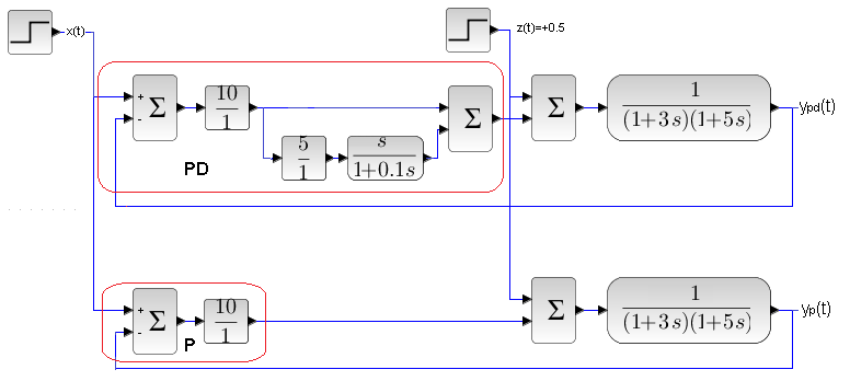

Fig. 14-12
Comparison of PD and P
The same objects G0(s) and the same signals x(t) and z(t). I wonder who will win the PD versus P match?
Chapter 14.6.5 Comparison of PD and P control

Fig. 14-13
Who is better PD or P?
When it comes to x(t) then clearly ypd(t) is better than yp(t). The ypd(t) signal reaches the steady state almost immediately, and yp(t) only after 20 seconds. In addition, with overregulation. How to explain the positive differentiation effect in PD? During the unit step x(t) , the PD controller gives a big “differentiating” kick from D. Then ypd(t) increases very quickly. We are afraid of overregulation. But then there will be an “inhibiting” effect of the D component, because ypd(t) enters with a minus on the controller from PD. This will prevent overregulation.
In the steady state there is a draw due to the fact that for PD the derivative component disappears. That is, P and PD do not provide zero error. In PD, however, the dynamics are much better.
And the reaction to a positive disturbance z(t)=+0.5 in 30 sec?
And here’s the problem. Because, although with overshoots, yp(t) seems better than ypd(t). As a PD attorney, I would emphasize the “seems.” However, this is not convincing for the judge and the audience. Then I will say this. Here, the settings Kp = 10 and D=5sec were selected due to the optimal response to the input x(t), and not the disturbance z(t). However, believe that you can tune PD so that the response to x(t) will be a little slower, but still much faster than for P. In ro, the response to the disturbance z(t) will be much better.
Chapter 14.6.6 Conclusions
Although both adjustments do not provide zero steady-state error, the PD conttrol is much faster than the P. It should be used when speed of response is more important than accuracy. Imagine you are taking part in a radio-controlled model car race. Do you want it to drive exactly to the cm on the designated track? Is it about not getting off the track at all?

Chapter 14.7 PID-Proportional-Derivative-Integral Continuous Control System.
Chapter 14.7.1 Introduction
We already know that:
– P control, and especially PD control, responds quickly to a unit step value x(t), but the steady-state e(t) error  is always non-zero.
– PI control ensures zero e(t) error, but the process is slower than for P control, and even more so for PD control.
The method imposes itself. You need to add a derivative component D to the PI controller. It will turn out that the response will be faster. In addition, the system will be more stable. And what does this mean? That, for example, you can increase the Kp gain of the controller, which will make the waveforms even faster. We will start by examining the structure of a PID controller
Chapter 14.7.2 Response of the PID controller to the step signal x(t).
It is not yet a controller because it does not perform its most important function, i.e. comparison e(t)=x(t)-y(t). For now, the input is only x(t) and we study the dynamics itself.

Fig.14-14
PID unit
Kp=1 Ti=10 sec. Td=1 sec
3 control components are implemented:
-proportional sP(t)
-integrating sI(t)
-differentiating sD(t)
The input signal is unit step x(t).
The controller’s sPID(t) signal is the sum of the sP(t), sI(t) and sD(t) components.
The Proportional component sP(t) is x(t) since Kp=1.
The Integrating component sI(t) increases at such a rate that after time Ti=10 sec it equals the proportional component sP(t). Here in the 13th second, which is invisible because the experience ends in the 10th second.
Differentiating component sD(t) – In the 3rd second, there is a unit step in x(t), i.e. at this time the speed is infinitely great. And this would be sD(t) for the ideal differentiator D. And it is real! That is, “flattened” by the inertial unit with time constant Td=0.1 sec. Due to disturbance, the ideal derivative unit D is rarely used.
The sP(t) and sI(t) components are easy to interpret when the input signal x(t) is a unit step. It is worse with sD(t) because for t=3 sec the signal speed is infinitely high. Therefore, let us analyze the PID again as x(t) increases linearly.
Chapter 14.7.3 PID control with disturbance z(t)=+0.5 z(t), Kp=10, Ti = 7 sec, Td=1.5 sec

Fig.14-15
The controller is optimal with respect to x(t). The disturbance z(t)=+0.5 will appear in 30 seconds. Up to 30 seconds, there is only a reaction to x(t). Initially, the disturbance z(t)=+0.5 caused the y(t) signal to increase, but then the sPID(t) control signal “forced” y(t) to return to its previous value, i.e. to y(t)=1. This corresponds to the appropriate reduction of the error e(t) to 0. It is beautiful to see how the PID controller responded in steady state to additional heating z(t)=+0.5 by cooling sPID(t)=-0.5. The D component improves the dynamics of the waveform.
Note!
In response to the disturbance z(t)=+0.5, the control signal sPID(t) coincides in the steady state with the disturbance z(t)=+0.5.
Ch. 14.7.4 Comparison of P, PD, PI and PID controllers
We will compare the P, PD, PI and PID control by simultaneously giving this same unit step x(t) to 4 control systems controlling the same object as in Fig. 14-15. Optimal controller settings have been selected.

Fig.14-16
Diagram for comparison of P, PD, PI and PID control
We guess which regulation is best.

Fig.14-17
Comparison of P, PD, PI and PID controllers
The black yP(t) regulation P is the worst. It has the most oscillation, lasts a long time and does not provide zero error.
The green yPD(t) of the PD control has the best dynamics – an almost rectangular response. It also does not provide zero error.
Blue* yPI(t) of PI control ensures zero error, but long control time and oscillations.
Red yPID(t) has the most advantages. Zero error, short control time and low oscillation.
Compare especially the effects of the work of the fancy PID controller and its poor relative the PID controller.
* You can’t really tell it’s blue.