Scilab

Chapter 12. Xcos-Transmittances, Operator Calculus and Differential Equations

Chapter 12.1 Introduction
In Chapter 11 we learned the basic dynamic units. The so-called transmittance G(s). This is an extension of the concept of gain K. You already associate G(s) with its response, e.g. to a unit step. And so in the Inertial unit G(s)=K/(1+sT) you know what the parameters K and T do. And s itself? What the devil? You may skip the topic on your first attempt. It just is and that’s it. And G(s) is something that reacts this way and not differently to a unit step or a “ramp”. A more serious look at G(s) is as the gain K depending on the frequency of the sine wave introduced to the input. A kind of frequency response. In the proportional term G(s)=K the relation is simple y(t)=K*sin(ωt). For each frequency/pulsation, the gain K is constant. Also the sine wave y(t) is in phase with sin(ωt). However, for “real” G(s), which is governed by differential equations, the amplitude and phase of the sine wave change with frequency. Typically, the amplitude decreases and the phase lags.
You can find more in the Automatic course, chapter 18.

Chapter 12.2 Transmittance G(s) and the differential equation
Chapter 12.2.1 Introduction
What is s in the transmittance G(s)? In Operational Calculus – in other words, in Laplace Transforms, each time function f(t) corresponds to its transform F(s) and vice versa, i.e. f(t)<==>F(s).
E.g. for a unit step of 1(t)<==>1/s.
The Operational Calculus has one nice feature
If f(t)<==>F(s) then f'(t)<==>s*F(s)
That is, the transform of the derivative f'(t) is the product s*F(s).
If it did not have this feature, there would be no Operational Calculus.
While it is impossible to write a simple relation in an object as simple y(t)/x(t) (because it would change over time t), it can be written as a ratio of 2 transforms G(s)=y(s)/x(s).

Chapter 12.2.2 Inertial Unit and the differential equation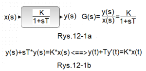

Fig.12-1
Relation between the differential equation and the transfer function G(s) of the inertial unit
Fig.12-1a
Transmittance G(s) of the inertial unit as G(s)=y(s)/x(s)=K/(1+st)
Fig.12-1b
The relationship between the operator equation of the inertial unit and its differential equation.
Chapter 12.2.3 A more complicated transmittance and the differential equation
We have already shown that an object described by a simple differential equation
K*x(t)=T*y'(t)+y(t)
corresponds to the transmittance G(s) of the inertial unit with parameters K and T.
The figure below shows how the transmittance is created for a more complicated differential equation, e.g. 3rd degree.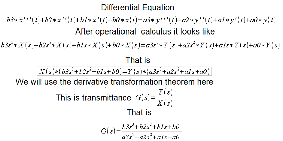

Fig. 12-2
So we see that the transmittance G(s) is a quotient where the numerator L(s) and the denominator M(s) are polynomials of the appropriate degrees. Usually, L(s) has a lower degree than M(s) and most often it is only L(s)=bo, in addition bo=1, and the denominator is the product of polynomials of the first or second degree.
In a similar way, a transfer function will be created based on a differential equation of any degree.
Let’s check the response of the G(s) to the step unit x(t) in Fig. 12-2 with specific parameters of the denominator M(s) and the numerator L(s).
M(s)–> a0,a1,a2,a3
L(s)–> b0,b1,b2,b3

Fig. 12-3
We see higher derivatives mixing up over time. Especially since the coefficients for these derivatives are small. What if they were big. Scary to think!
For most transmittances, the steady-state gain K can be easily determined. It is simply an free expression because bo=1.25 in the numerator of the transmittance, assuming that the free expression in the denominator ao=1. If ao is different from 1, divide the numerator and denominator by ao.
Of course, this is the case when G(s) concerns stable systems. Not ones where any disturbance causes G(s) to become a generator. You know a lot about the transmittance response G(s) unit step 1(t).
The output y(t=2)=0, which is obvious, and that in the steady state y(t)=bo=K. But what happens in the transition state (“in between”), i.e. for t=2…15 sec? The remaining transmittance parameters are responsible for this. These are the coefficients a1, a2, a3 and b1, b2, b3, the specific values of which are visible in the transmittance G(s) in Fig. 12-3