Scilab

Section 11.2 How will we study basic dynamic units?
Chapter 11.2.1 Introduction
We are surrounded by dynamic units – proportional, inertial, oscillatory, integrating, etc…. I.e. For an automatics engineer, the lever is a proportional, an inertial in the first approximation, and a multi-inertial unit unit in the second approximation. And the weight on a spring is an oscillating spring. This means that everyone looks at reality through the prism of their experiences or profession. By the way, a fireman was asked, what the difference was between a cello and a violin. Answer-the cello burns longer. Let’s stop the jokes. The most important thing is that you associate the transmittance G(s) with something obvious. With the response y(t) of the object to the input x(t) – specifically to a step unit.

Chapter 11.2.2 Universal Diagram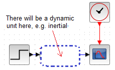

Fig. 11-1
Universal Scheme
This is how we will study the basic dynamic units in Chater 11.3…1.11.

Chapter 11.2.3 More about the Universal Schema
When examining the basic dynamic units, starting from Proportional and ending with Inertial with delay, the diagram will always be as in Fig. 11-1, more precisely in Fig. 11-2. We will only change the denominator (mostly) and numerator of the CLR unit and, less frequently, as necessary, the parameters of the remaining units.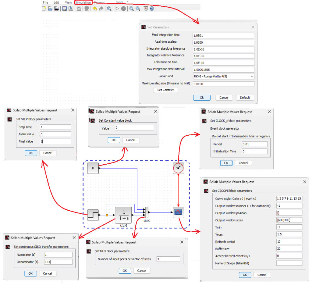

Fig.11-2
Universal Xcos scheme for testing dynamic units.
Most often it will be like this:
– Universal Transmittance CLR – This is the Inertial Unit that we will modify, including transforming into other units, in Chapter 11.3…11.
– The input is a unit step from 0 to 1 and a delay of 1 sec*
– Oscilloscope settings Ymin=-1, Ymax-+1.5, refresh time=10 sec
– Block setting const=0 (for plotting the x-axis of the chart)
– Clock setting Period=0.01sec Initialization time=0sec
– Multiplexer setting=3 inputs
– Settings in the “Simulation” tab – Final integration time=10 sec, real-time scaling=1, Solver kind=RK45 Runge-Kutta4(5)_
The simulation parameters can be obtained by double-clicking the Simulation tab with the left mouse. We enter a decimal number, e.g. 10, which will automatically change to scientific notation, i.e. 10–>1.0E01.
The parameters of the remaining blocks can be obtained by clicking them twice with the right mouse. The above windows will then open with smaller windows in which you can enter the appropriate parameters. For example, in the Set_CLOCK_c clock window the parameters Period = 0.01 and initial time 0 in seconds are entered.
* When testing the Differentiator, the input will be a ramp signal instead of a Unit Step.

Chapter 11.2.4 How to create a Universal Schema?
That is, from Fig. 11-2. We will use it to create diagrams in chapter 11.3…11.
This will be best demonstrated by an animation.

Fig.11-3
Creating a Universal Schema
You see the final state of creating the schema, where I saved it in a folder as …xcos/czlon_pattern. It’s obscured by the Save As window…but you’ll see it in the blue “dashed” box in Fig 11-2.
The animation will feature subsequent stages of creating the Universal Scheme.
1. Initial state with open windows
–Palette browser – it opens Recently used blocks – Convenient for the user, because recently used blocks appear here.
–Untitled-Xcos – in it we draw block diagrams by downloading blocks from specific palettes of the Palette Browser.
2. In the Untitled blocks window, select the File/New Scheme tab with the left mouse (this takes a short time in the animation!)
3. From the Sources palette, use the left mouse to move the –Step_Function, Const, Clock_c blocks to Untitled blocks,
4. From the Sinks palette, use the left mouse to move the CSCOPE block to Untitled blocks
5. From the Signal Routing palette, use the left mouse to move to Untitled blocks MUX multiplexer
6. From the Continuous Time Systems palette, use the left mouse to move the CLR transmittance to Untitled blocks
7. Entering 0 into the Const block
8. Entering 3 into the MUX block (3 inputs)
9. Draw the connections with the left mouse
10. Now the job is for you. Check the parameters of the remaining blocks and the Simulation tab. They must be as shown in Fig. 11-2. If not, change them.
You know how to do it. Click with the right mouse, etc… Simulation tab with the left mouse, etc…
11. Saving the file under a name in a folder, here …xcos/czlon_wzor. You save it wherever you want.
The last point is very important! Will you save a lot of work in chapters 11.3…11.?

Chapter 11.3 Proportional Unit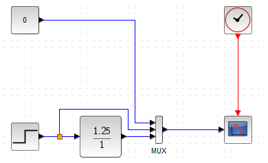

Fig.11-4
Proportional Unit with gain K=1.25
The simplest dynamic unit. The output y(t) is related to the step input x(t)=1(t-1)* by an algebraic (not differential!) equation y(t)=K*x(t). Here K=1.25. Immediate response to entry. You wouldn’t want to be in a car that reacted with such speed v(t) to pressing the gas pedal x(t). Air catapult acceleration is a small beer.
* 1(t-1) is a unit step shifted in time by 1 sec.
The diagram in Fig. 11-4 will be obtained as follows:
– Downloading the unit_pattern file from the ...xcos folder, which I saved in p.10 of the animation Fig.11-3. You could have written it down somewhere else.
– Changing the CLR transmittance block parameters from 1/(1+s) to 1.25/1
– Scheme unit_pattern, you can save it or not. At most in the future unit_pattern there will be a different CLR transmittance. I guess you can do it yourself now.
I added an animation just in case. When examining subsequent dynamic units, it will no longer be there.

Fig.11-5
Realization of the Proportional Unit G(s)=1.25 and its response to a unit step.
The answer is immediate. Compare the output y(t) with the input x(t). You can see that y(t)=1.25*x(t).
1. Download the unit_pattern schema
2. Change of CLR transmittance from 1/(1+s) to 1.25/1
3. Press “Start” and watch the simulation
x(t)-green
y(t)-red
The transmittance of the proportional unit is simply G(s)=K, where K is the gain here K=1.25.
If you have eagle eyes, you can see the time waveforms y(t) and x(t) and their steady states y and x. For the Proportional Unit, which responds instantly, y(t)=y and x(t)=x and the gain K=y/x.
In everyday life, almost all objects you deal with are proportional units. At least at first glance.
Examples:
Swing
The change in the position of the left saddle x(t) corresponds to the same shift only in the opposite direction
right saddle y(t), therefore y(t)=-1*x(t). So it is a Proportional Unit with a gain of K=1

Amplifier
Output voltage y(t)=K*x(t) when the input is input voltage x(t). The K parameter is the gain
Transformer
Amplitude of the output sine wave voltage y(t)=K*x(t), when the input is the amplitude of the input sine wave voltage x(t).
The K gain is called gear.
Now what does “At least at first glance” mean? Well, we don’t see transition states,
which will only become visible upon closer analysis.
The transformer amplitude will not change immediately, only after e.g. 1 second.
Amplifier–>On a good oscilloscope you can also see that the output y(t) will not change immediately
Swing–>This is a more difficult topic. But if we take into account the dynamic deflections of the beam with rapid changes in x(t)…

Chapter 11.4 Inertial Unit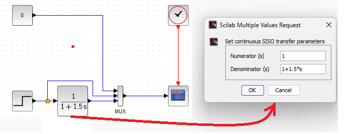

Fig.11-6
Inertial Unitt with gain K=1 and time constant T=1.5 sec
It also shows how the transfer function 1/(1+1.5s) was entered. Note that you entered 1.5*s (with an asterisk) and not 1.5s (without an asterisk).
After clicking on the “Start” triangle in the top tab of Xcos, you will receive this waveform.

Fig.11-7
Response y(t) of the Inertial Unit 1/(1+1.5s) to a unit  step x(t)
The parameter T=1.5sec will be obtained from the tangent, and the gain K=y/x, where y and x are the fixed values of the output y(t) and x(t). If G(s) had the form, e.g. G(s)=2/(2+3s), then the numerator and denominator should be divided by 2 and we would get G(s)=1/(1+1.5s) in which the  parameters are visible K=1 and T=1.5sec of the Inertial Unit 

Chapter11.5  Double-Inertial Unit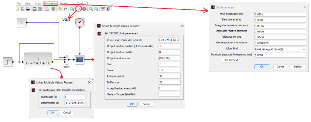

Fig.11-8
Two-inertial unit with gain K=1 and time constants T1=2 sec and T2=5sec
With these parameters we expect longer time waveform. Therefore, we will change the Oscilloscope and Simulation tab settings to a run time of 30 seconds. After entering the parameters of the CLR block, it had to be stretched using the classic Windows method.
After clicking the “Start” triangle in the top tab in Xcos, you will receive a waveform.
Note:
The Real time scaling should be set 1 and not 0 as in the Set Parameters in Fig.11-8

Fig.11-9
Response y(t) of the Double Inertial Unit G(s)=1/(1+2s)(1+5s) to a unit step x(t)
The K=1 gain can be easily calculated from the chart as the ratio of the set values K=y/x. It’s not so nice with the T1 and T2 parameters.
There’s probably a method, but let’s leave it alone. There is a characteristic inflection point in the graph near the inscription y(t).
The Double-Inertial Unit is a series connection of two Inertial Units, the Three-Inertial element is a series connection of three Inertial Units etc…

Chapter 11.6 Ideal Integrating Unit
Previously, we changed the block settings and Simulation tabs. Therefore, go back to the previous ones in Fig.11-2.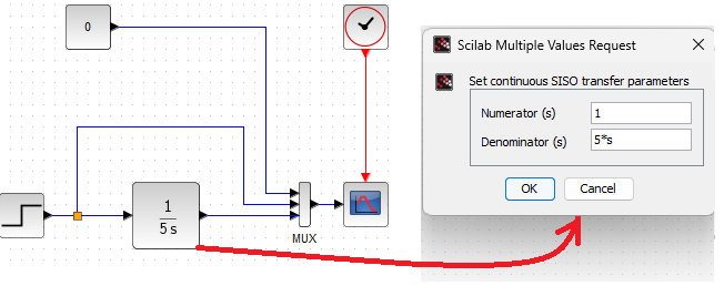

Fig.11-10
Integrating Unit with integration constant Ti=5 sec
The integration constant Ti is the time after which the output signal y(t) reaches the input value x(t) of a step unit.

Fig.11-11
Response y(t) of the Ideal Integrating Unit G(s)=1/5s to a step unit  x(t)
Notice, that after a time of Ti=5sec, the output signal y(t) has become equal to the step unit x(t).
And what will be the waveformo the “ram” y(t), e.g. for twice as small, i.e. Ti=2.5 sec?

Fig.11-12
Response y(t) of the Ideal Integrating Unit G(s)=1/2.5s to a unit step x(t)
The process is 2 times faster. Draw your own conclusions.
An example of an integrating unit is an ideal DC motor. I.e. with low mass and inductance. In short, like any ideal, there is no such thing in the world. Then the response of its shaft angle α(t) to the DC voltage step u(t) will be as above. Let me remind you that α(t) can be greater than 360º.

Chapter 11.7 Real Integrating Unit, i.e. with Inertia
And how will a real DC motor react if the rotor has inertia and the winding has inductance?
Of course, with a certain lethargy, i.e. with inertia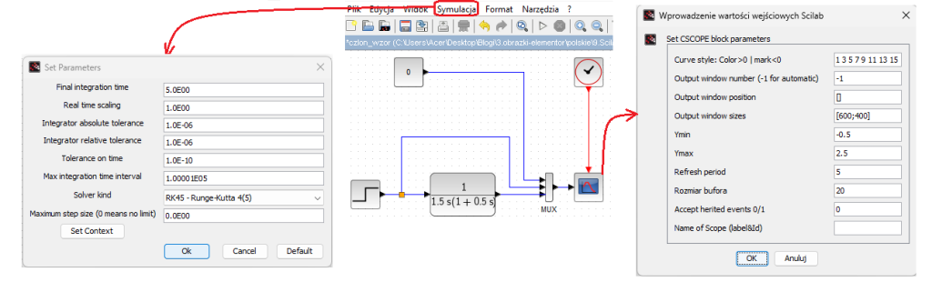

Fig.11-13
Real Integrating Unit Ti=1.5sec and T=0.5sec
As a series connection of the integrating unit Ti=1.5 sec with the inertial element T=0.5 sec.
Note:
Due to the different time range of the waveform than before, change the oscilloscope settings and the Simulation tab as shown in the above figure.

Fig. 11-14
Response y(t) of the Integrating Unit G(s)=1/2.5s to a unit step x(t).
It is shown how to read the integration time Ti and the inertia time constant T from the graph.

Integrating unit with inertia as a series connection
So like this.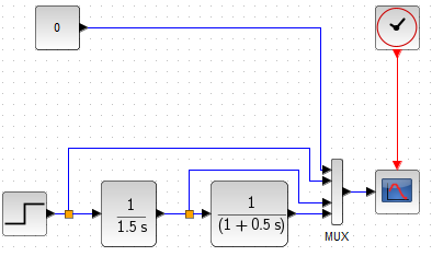

Fig. 11-15
This approach will allow us to notice something.

Fig.11-16
How the graph of the integrating unit with inertia is shifted relative to the integrating unit.
Here it is clearly visible that the inertial component is shifted parallel to the right relative to the ideal one by the inertia constant T=0.5 sec.

Chapter 11.8 Ideal Differentiator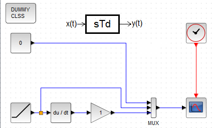

 Rys 11-17
Ideal Differentiator
For various reasons, we will not modify the CLR block, but we will call a separate du/dt differentiation unit from the Continuous Time Systems palette. I also recommend downloading the DUMMY CLSS unit from there. I won’t go into why, but Scilab won’t scream that something’s wrong. The diagram shows that the parameter of the differentiation constant Td is Td=1 (or more precisely, Td=1sec). After pressing “Start” you will know it is about. 

Fig.11-18
Response of the Ideal Differentiator sTd when Td=1sec.
The answer is similar to Fig. 11-11, only “a rebours”. What was the entry is the exit. A unit step signal cannot be used as input for the Differentiator . Because what is the derivative at the moment of the step? Infinitely great! It is difficult to derive, for example, the value of the Td parameter from this. What if the input is a linearly increasing signal? In other words, “a ramp” No problem. This is the time Td after which the output signal y(t) equals the “ramp” value. And this is regardless of the speed of growth of the “ramp” x(t). So let’s check if Td=2sec? Change the value of the amplifier k=1 from Fig. 11-17 to k=2.

Fig. 11-19
Response of the ideal derivative sTd when Td=2sec.
The output signal is twice as large as we expected. Regardless of the slew rate of the input signal x(t).

Chapter 11.9 Real Differentiator Unit, i.e. with Inertia.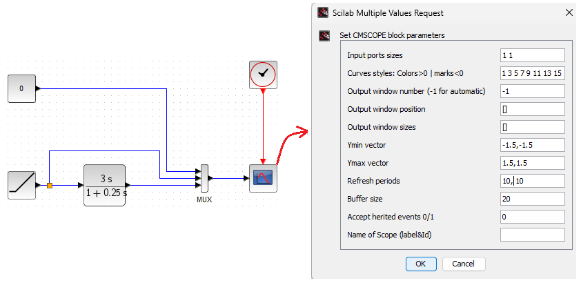

Fig.11-20
Real Differentiator Unit and oscilloscope settingd
We used the CLR element again and modified it accordingly.

Fig.11-21
The response of the Real Differentiator to a linearly increasing signal x(t) when Td=3sec and T=T0.25sec.
The parameter Td=3sec is the time for the steady output signal y(t) to equalize the input “ramp” x(t). Notice that the entry is a ramp, not a step!

Chapter 11.10 Oscillation Unit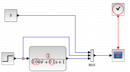

Fig.11-22
Oscillation Unit in normalized form. I.e. one in which the free expression in the denominator=1
We will calculate the parameters based on the values in red circles:
1-->Gain k=1 (denominator numerator)
0.04–>(o.2²=0.04)–>Oscillation period Tosc=2*π*0.2≈1.256sec
0.1—>(2*q*0.2=0.1–>q=0.25)–>Attenuation q=0.25
Originally, the fraction form could be unnormalized, e.g. 3/(0.12s+0.3+3).
If we divide the numerator and denominator by the free expression, i.e. by 3, we will obtain a standardized form.

Fig.11-23
Previously, we calculated the parameters of the oscillation unit from the red circles. We can also calculate the parameters from the chart.
We calculated the gain k=1 as k=y/x=1/1=1 when y and x are steady states
The oscillation period Tosc≈1.3sec is slightly larger than Tosc=1.256sec calculated in Fig. 11-22.
The attenuation parameter q can also be calculated, but let’s leave it alone. This is a Scilab course, not a Control Theory Course.
You can find more in Chapter 7 of the Automatics course.

Section 11.11 Delay Unit and Substitute Transmission
Chapter 11.11 .1 Introduction
So far, you have learned most of the typical dynamic units described by transmittance, or if you prefer, by differential equations. It may be a furnace, a rocket, a chemical reactor whose input is the flow of e.g. a alkali and its output is the pH coefficient. Each transmittance is different. For convenience, automatics engineers invented the so-called equivalent transmittance, which is a series connection of the Delay and Inertia units. And what’s that for? In chemistry, for example, many objects are described as multi-inertial. They react to the step unit by “accelerating”, then there is the maximum speed, which gradually decreases until it reaches a steady state. From the waveform itself, we can easily determine the gain K=y/x where y, x are steady values. And the time constants T1,T2,…Tn? This is a high driving school. Therefore, an equivalent transmittance was invented, which has only 3 parameters. Gain K, Inertia T and Delay To. They are easy to determine from the chart. In addition, for these three parameters, wise people have long ago selected the optimal settings of PID controllers, so that the response of the closed system is in some respect the best.

Chapter 11.11 .2 Delay Unit exp(-sTo)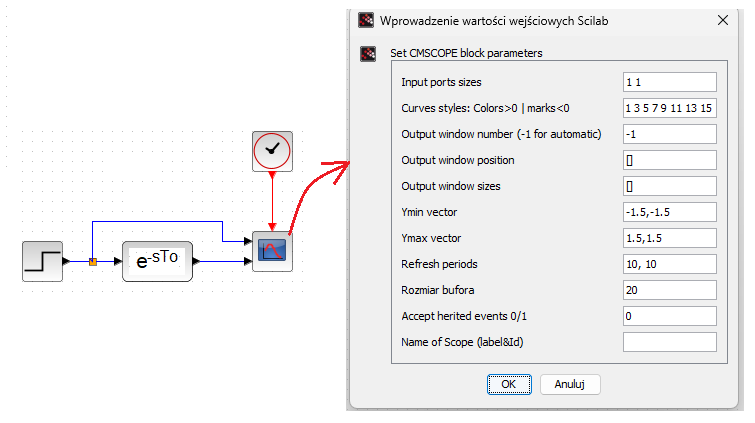

Fig.11-24
Delay Unit exp(-sTo) and 2-channel oscilloscope settings
To=3sec i.e. exp(3*s)
Note.
The s symbol in exp(3*s) is not a second! This is a complex number s. More on this in the next chapter.
You will find the Delay Unit in the Continuous Time Systems palette as the TIME_DELAY block

Fig.11-25
Response of the delay unit exp(-4*s) to a unit step.
The output is clearly delayed by 4 seconds.

Chapter 11.11.3 Substitute Transmittance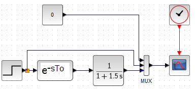

Fig.11-26
Substitute Transmittance as a series connection of the Delay and Inertia Unit.

Fig.11-27
Equivalent transmittance G(s) with parameters
K=1, To=0.5sec, T=1.5sec
Gain K=1, delay To=0.5sec and T=1.5sec “as a tangent” are obvious.