Scilab
Chapter 10 XCOS-Inputs and outputs, i.e. generators and oscilloscopes
Chapter 10.1 Introduction
Every technologist designing an industrial installation or electronic amplifier must know, what the response of what he is designing is to the input. Modeling in Xcos involves downloading from the so-called pallets of appropriate blocks and drawing connections between them.
Generators and oscilloscopes belong to these blocks and are included:
Generators – in the Sources palette
Oscilloscopes – in the Sinks palette
Chapter 10.2 Input-unit step, Output single-channel oscilloscope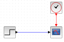
Fig.10-1
Input-unit step, output-single channel oscilloscope
I wonder what the unit step will look like on the oscilloscope. But first you need to model the above. diagram in Xcos
Fig.10-2
Construction of the diagram from Fig. 10-1 in Xcos and its recording on a single-channel oscilloscope.
The animation shows the final state of the animation, i.e. the state of the oscilloscope.
The animation shows:
1. Download the step unit block from the Sources palette
2. Download the CSCOPE block (single-channel oscilloscope) from the Sources palette
3. Downloading the CLOCK_c block (clock) from the Event Handling palette*
4. Drawing connections
5. Click the “Start” triangle. A small chart window will appear.
The result is a unit step recorded on the oscilloscope.
Of course, you can enlarge the small window as much as possible by clicking the appropriate Windows button.
I advise you to save the diagram somewhere. It will be useful later, e.g. in Fig. 10-8
Chapter 10.3 Setting clock, oscilloscope and unit step parameters
The unit step parameters in the oscilloscope Fig. 10-2 are not optimal.
What don’t I like?
– The unit step has a range of 0…1 and the range on the oscilloscope is –15…+15
– The unit step is not ideal because it increases linearly, why?
– The time range of the unit step is 0…30 sec. Just 0…5 sec. By this time everything had settled down!
Let’s tinker with the settings by right-clicking on the appropriate blocks.
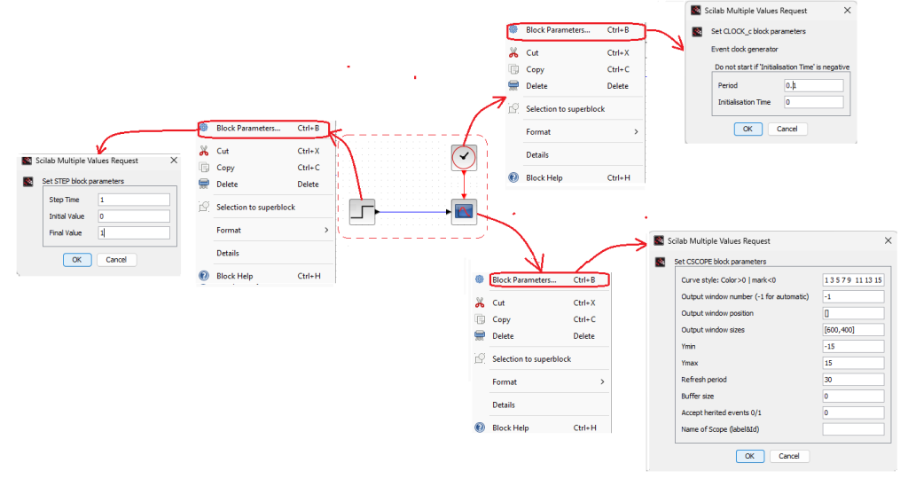
Fig.10-3
Setting the clock, oscilloscope and unit step parameters.
Clock_c (Clock)
A clock is used to quantize time, which in the classical sense is continuous. And in Xcos it changes every arbitrary quantum period. Nothing easier. The smaller the period, e.g. a millionth of a second, the better. But then the number of calculations increases. And since the so-called recursion, errors accumulate. Not only do the calculations take longer, but they are less reliable. A certain period, not too long and not too small, is optimal. What? I’m not a mathematician and I use intuition. When I see that the waveforms change relatively evenly over time, e.g. 5 seconds, I will initially try to give a period of e.g. 0.1 sec. When I see that Xcos has calculated clearly wrong, I will reduce it to 0.01 sec and check “if it has improved”. Mostly yes, but not always.
Let’s get back to the setting. I right-click on the clock block and go to the selection window. Here I click Settings Block–>Set CLOCK_c. I set the period here to 0.1 sec and the initial state to 0. This is how the period of 0.1 sec was set in Fig. 10-1. It’s probably too big, because the jump looks like a trapezoid. In the next experiment I will give 0.01 sec.
CSCOPE (single channel oscilloscope)
I right-click on the oscilloscope block and go to the selection window. Here I click Settings Block–>Set CSCOPE block parameters and I can set, among other things:
-line color of different waveforms – Useful when there are several waveforms in a single-channel oscilloscope. Strange in single channel several waveforms? But there is a possibility.
-Dimensions of the waveform window
-Ymax
-Ymin
-Screen refresh period
STEP_FUNCTION (Unit Step)
Settings
– Delay (here 1 sec)
– Initial value (here 0)
– Final value (here 1)
Well, let’s change the settings to make it nicer.
Fig.10-4
Chart after changing block parameters.
See in the animation how I did it.
1. Changing the quantization period in the clock from 0.1sec* to 0.01sec. The steepness of the unit step should improve
2. Changing the scope of the oscilloscope screen from -15…+15 to -1…+2. Enlargement, i.e. you can see more details.
3. Changing the delay in a unit jump from 1 sec to 1.5 sec, the initial value from 0 to 0.5 and the final value from 1 to 1.5.
So the new step unit will be 0.5…1.5. Why, if a unit step of 0…1 is the most natural? Just so you can play with the settings window.
*Your initial clock and other settings may be different.
Note
The changes I made by right-clicking on the blocks are what I expected.
I’m still lucky, that the experiment is long enough. Lasts from 0…30 sec. Why take so long if nothing happens for 2 seconds?
The experiment time
We can change it by right-clicking on the “Simulation” tab of the Xcos window. You can also change other parameters.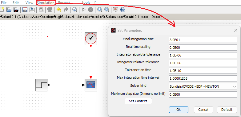
Fig.10-5
Simulation Window
A very important window in which we set the most important calculation parameters of XCOS, mainly related to integration.
You can set 7 parameters in 7 windows. For 6 we enter a decimal number which will automatically change into scientific notation.
The most important are:
1. Final integration time.
Simpler–>experiment time. Here 30 sec. otherwise 3.0E01 in the scientific version.
2. Time scaling
0=0.0E00-The chart appears “immediately”. More precisely, immediately after the simulation calculations.
1=1.0E00-Real-time graph. E.g. When the capacitor in the RC system charges for 5 seconds, the graph on the screen also lasts 5 seconds.
As if we were observing a real RC system! I almost always use this method.
3. Solver kind
Without going into details, Xcos solves differential equations numerically, relying mainly on the calculation of the integral, i.e. the area under a function of, for example, time. The more precisely we calculate it, the more accurately we will solve the differential equation. In this window we choose the integration method. There are 8 of them here. So which one should you choose? I will answer briefly and to the point. I don’t know, but I choose RK-Runge-Kutta 4(5). People use it a lot, and it’s a cool name. Kind of like bunga-bunga. A little more seriously. If you suspect that the resulting simulation waveform is not out of the realm of dreams, try the other methods.
Fig.10-6
Chart after the final change of block parameters
1. Changing the screen refresh period from 30 sec to 5 sec
2. Changing the delay in a unit step from 1.5 sec to 1 sec and the amplitude range from 0.5…1.5 to 0…1. That is, back to a typical unit step.
3. Changing the Final Integration Time from 30 sec to 5 sec after right-clicking the Simulation tab. It is obvious that it should be the same as the Screen Refresh Period from p1, i.e. 5.
4. In the same window, I set Real-time Scaling from 0 to 1. This course, unfolding before our eyes, reflects the dynamics of the process more than an “instant” graph like in the book. I used this principle in this course and in others, including Automatics.
As a result, we received a beautiful, almost rectangular graph with a “horizontal” range of 0…5 sec and a “vertical” range of -1…+2.
Chapter 10.4 Inputs – square wave, unit step and sine wave, Output single-channel oscilloscope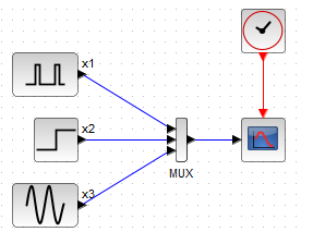
Fig. 10-7
Inputs – square wave, unit step and sine wave, output single-channel oscilloscope.
Square wave, unit step and sine wave generator are obviousl. Single-channel oscilloscope too. We can guess the role of the MUX block. Also new are x1, x2 and x3 text blocks. Let’s create and check this diagram.
Fig.10-8
Construction of a diagram with 3 input signals x1, x2 and x3 on a common screen of a 1-channel oscilloscope
1. Download the diagram most similar to Fig.10-7. In my case it is Fig. 10-1, which I previously saved in the folder as …xcos/Scilab10-1. If you don’t have an ancestor, build the schema from scratch. A construction engineer would starve if he started every project from scratch.
2. Download square wave and sine wave generator blocks
3. Delete unnecessary connection
4. Downloading the MUX multiplexer and changing the number of inputs from 2 to 3
5. Connecting blocks with lines
6. Change the parameters of individual blocks with the “right mouse” -> see *Note
7. Retrieving text blocks from the Annotations palette (the palette has only 1 block!–> TEXT_f). By double-clicking with the left mouse, you select and change the text. Placement of texts x1, x2 and x3 at the appropriate generators.
*Note
There will be some boring text here, but digest it. It will be useful when setting Xcos parameters.
I want 5 square wave generator periods, 1 spike and 1 sine wave generator period to be displayed in 5 seconds.
This is why:
1. The oscilloscope has a previously set refresh time of 5 seconds and Ymin=-1 and Ymax=+2. In the Simulation tab, the integration time is also 5 sec and real-time scaling=1. This means that the graph will expand for 5 seconds. As if you were observing a real experiment in a laboratory!
2. Square wave generator settings
-Delay 0
-Pulse fill 50%
-Period 1 sec
-Amplitude 1
3. Settings of the unit step generator
– Delay 1 sec
– Initial value 0
– Final value 1
4. Sinusoidal generator settings
– Amplitude A= 0.75
– Pulsation ω=1.257rad/sec–>Corresponds to the period T=2π/ω=5sec
The colors of the x1, x2 and x3 waveforms correspond to the colors 1,3,5 of the waveform lines in Fig. 10-3 from the oscilloscope setting–>black, green, red.
Chapter 10.5 Inputs – Square wave, unit step and sine wave, multi-channel oscilloscope output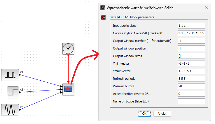
Fig.10-9
Inputs – square wave, unit step and sine wave, output multi-channel oscilloscope.
This is a modification of Fig. 10-7 in which we replaced the single-channel oscilloscope with a multi-channel one. The MUX mutiplexer is not needed.
By clicking with the right mouse, you will get a setting block similar to that in Fig. 10-3. And what are the differences?
– Added Input ports sizes window. Here, 3 1s mean 3 oscilloscope inputs for inputs x1, x2 and x3
– Ymin vector (-1,-1,-1) is the lower ranges x1min=-1, x2min=-1, x3min=-1
– Ymax vector (1.5, 1.5, 1.4) are the upper ranges x1max=+1.5, x2max=+1.5, x3max=+1.5
– Refresh periods (5,5,5) are times of 5 seconds for runs x1,x2,3
These settings will be used in the following animation Fig. 10-10
Fig.10-10
Construction of a diagram with 3 input signals x1, x2 and x3 on a common screen of a 3-channel oscilloscope
1. Download the diagram most similar to Fig.10-9. In my case it is the diagram from Fig. 10-7 which I previously saved in the folder as ..xcos/Scilab10-8.
2. Remove the MUX multiplexer. The connections also disappeared. Great, less work!
3. Downloading the CMSCOPE multi-channel oscilloscope from the Sinks palette
4. Removal of the “old” CSCOPE single-channel oscilloscope
5. Right-click the oscilloscope and enter the data from Fig. 10-9.
6. Drawing the connections
7. Clicking the “Start” triangle in the top tab
You will see 3 waveforms. Compare with the single-channel oscilloscope in Fig. 10-8.
The waveforms are the same, just on separate graphs.
After reading chapter 9, 10 you already have sufficient tools to build large and complex diagrams. For me, automatics engineer means Automatic Control Systems. Mechanics, electricians, chemists… will also find something for themselves. So let’s sail out of the port into the wide waters of the ocean of modeling physical phenomena.